4.2. Tutorial 2¶

Tutorial 2: Land Cover Classification of Sentinel-2 Images

4.2.1. Tutorial 2: Land Cover Classification of Sentinel-2 Images ¶

This tutorial describes the main phases for the classification of images acquired by Sentinel-2 Satellite. In addition, some of the SCP tools are illustrated.

We are going to classify the following land cover classes:

Water;
Built-up;
Vegetation;
Bare soil.

Following the video of this tutorial.

http://www.youtube.com/watch?v=FcETq8OWM0k

4.2.1.1. Data Download ¶

We are going to download a Sentinel-2 image provided by the Copernicus Scientific Data Hub. In particular we are going to use the following Sentinel-2 bands (for more information read Sentinel-2 Satellite):

Band 2 - Blue;
Band 3 - Green;
Band 4 - Red;
Band 5 - Vegetation Red Edge;
Band 6 - Vegetation Red Edge;
Band 7 - Vegetation Red Edge;
Band 8 - NIR;
Band 8A - Vegetation Red Edge;
Band 11 - SWIR;
Band 12 - SWIR;

TIP : In case you have slow internet connection you can download a subset of the image (about 50MB) from this link (© Copernicus Sentinel data 2016) which is the result of steps Data Download and Clip the Data.

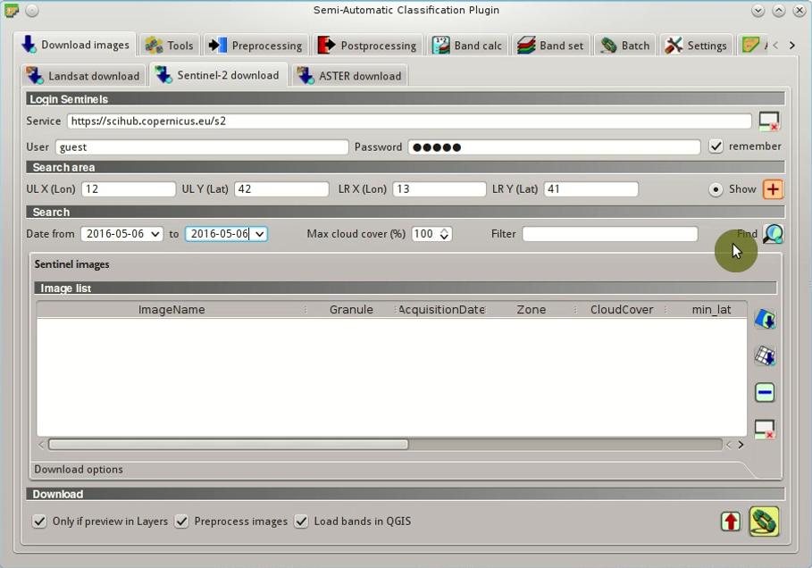
Start a new QGIS project. Open the tab Download images clicking the button in the SCP menu, or the SCP Tools, or the SCP dock. Select the tab Sentinel-2 download. We are searching a specific image acquired on May 06, 2016.

In Login Sentinels enter the user name and password for accessing data (free registration is required).

WARNING : The guest/guest account is not available anymore. Free registration is required. See https://scihub.copernicus.eu/news/News00097 .

In Search area enter:

UL X (Lon): 12
UL Y (Lat): 42
LR X (Lon): 13
LR Y (Lat): 41

TIP : In general it is possible to define the area coordinates clicking the button and drawing a rectangle in the map.

In Search set:

Date from: 2016-05-06
to: 2016-05-06

Search Sentinel-2 images

Now click the button Find and after a few seconds the image will be listed in the Image list.

Tip: download this zip file containing the shapefile of Sentinel-2 granules for identifying the zone; load this shapefile in QGIS, select the granules in your search area and open the attribute table to see the zone name.

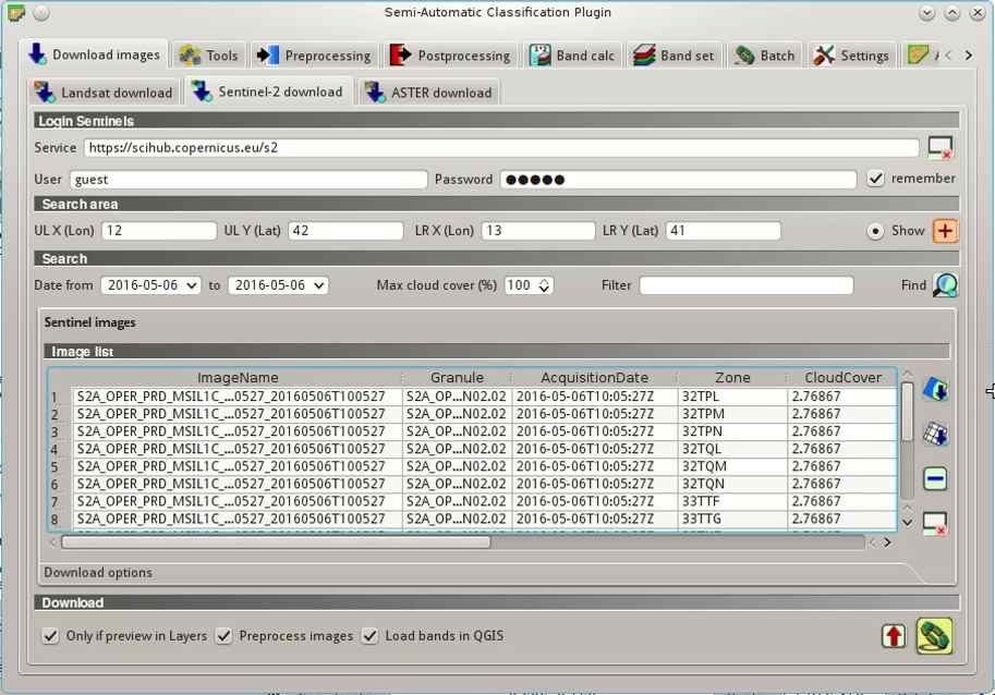
Sentinel-2 search result

In the result table, click the item T32TQM in the field Zone, which is the Granule S2A_OPER_MSI_L1C_TL_SGS__20160506T153005_A004552_T32TQM, and click the button . A preview will be downloaded and displayed in the map, which is useful for assessing the quality of the image and the cloud cover.

TIP : It is also possible to display the image overview (which is composed of several granules) with the button .

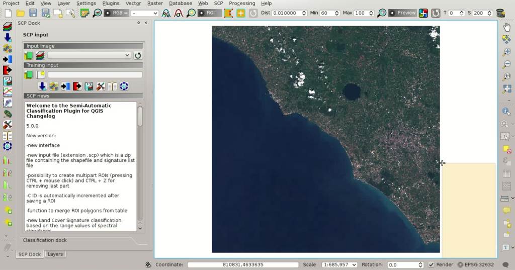
Image preview

Click the tab Download options and uncheck bands 1, 9, and 10. Also, uncheck the options Preprocess images (usually this should be checked, but for the purpose of this tutorial we are going to preprocess images in the step Automatic Conversion to Surface Reflectance) and Load bands in QGIS (because we are going to clip the images).

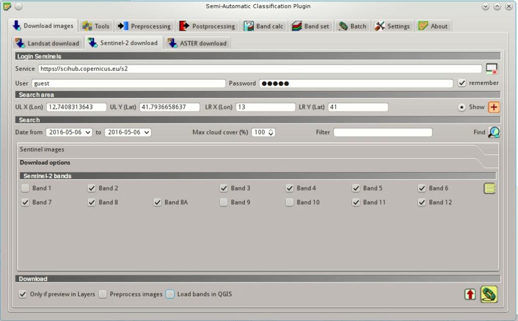
TIP : The option Only if preview in Layers allows for downloading only images in the result table which are loaded as previews in the map. It is convenient to check this option and remove the images previews in the QGIS layer list, leaving only the previews of images that one wish to download.

Selection of bands for download

In order to start the image download, click the button and select a directory where bands are saved (e.g. Desktop). The download could last a few minutes according to your internet connection speed (band size ranges from 30 to 90MB). The download progress is displayed in a bar.

After the download, all the bands and the metadata files are saved in the output directory.

Download of Sentinel bands

4.2.1.2. Automatic Conversion to Surface Reflectance ¶

Conversion to reflectance (see Radiance and Reflectance) can be performed automatically. The metadata file (a .xml file whose name contains MTD_SAFL1C) downloaded with the images contains the required information for the conversion. Read Image conversion to reflectance for information about the Top Of Atmosphere (TOA) Reflectance and Surface Reflectance.

In order to convert bands to reflectance, open the tab Preprocessing clicking the button in the SCP menu, or the SCP Tools, or the SCP dock, and select the tab Sentinel-2.

Click the button Directory containing Sentinel-2 bands and select the directory that should be named S2A_OPER_MSI_L1C_TL_SGS__20160506T153005_A004552_T32TQM. The list of bands is automatically loaded in the table Metadata. Also, the metadata information for each band is loaded (because the metadata file is inside the same directory).

TIP : If a Sentinel-2 image was downloaded directly from the site https://scihub.copernicus.eu and you want to convert images to reflectance using SCP, you should copy the .xml file whose name contains MTD_SAFL1C (included in the granule directory) and paste it inside the same directory of bands (files .jp2).

In order to calculate Surface Reflectance we are going to apply the DOS1 Correction; therefore, enable the option Apply DOS1 atmospheric correction.

TIP : It is recommended to perform the DOS1 atmospheric correction to the entire image (before clipping the image) in order to improve the calculation of parameters based on the image.

Uncheck the option Create Band set and use Band set tools because we are going to define this in the following step Create the Band Set. In order to start the conversion process, click the button and select the directory where converted bands are saved (e.g. Desktop).

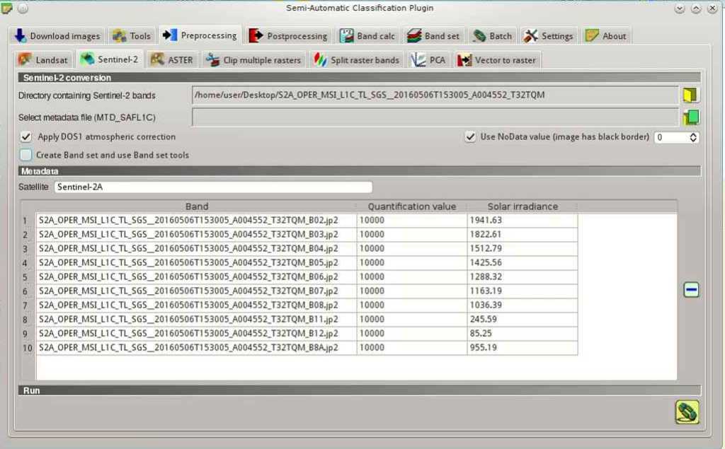
Sentinel-2 conversion to reflectance

After a few minutes, converted bands are loaded and displayed (file name starts with RT_). If Play sound when finished is checked in Classification process settings, a sound is played when the process is finished.

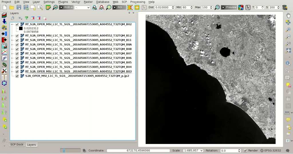
Converted Sentinel-2 bands

4.2.1.3. Clip the Data ¶

Sentinel-2 images have a large extent. In order to reduce the computational time, we are going to clip bands to the same study area as Tutorial 1: Your First Land Cover Classification. Open the tab Preprocessing and select the tab Clip multiple rasters.

Click the button to refresh the layer list, and check all the layers whose name starts with RT_ (the band number is at the end of the layer name).

Click the button and select an area such as the following image, or enter the following values:

UL X: 791810
UL Y: 4643020
LR X: 809750
LR Y: 4626230

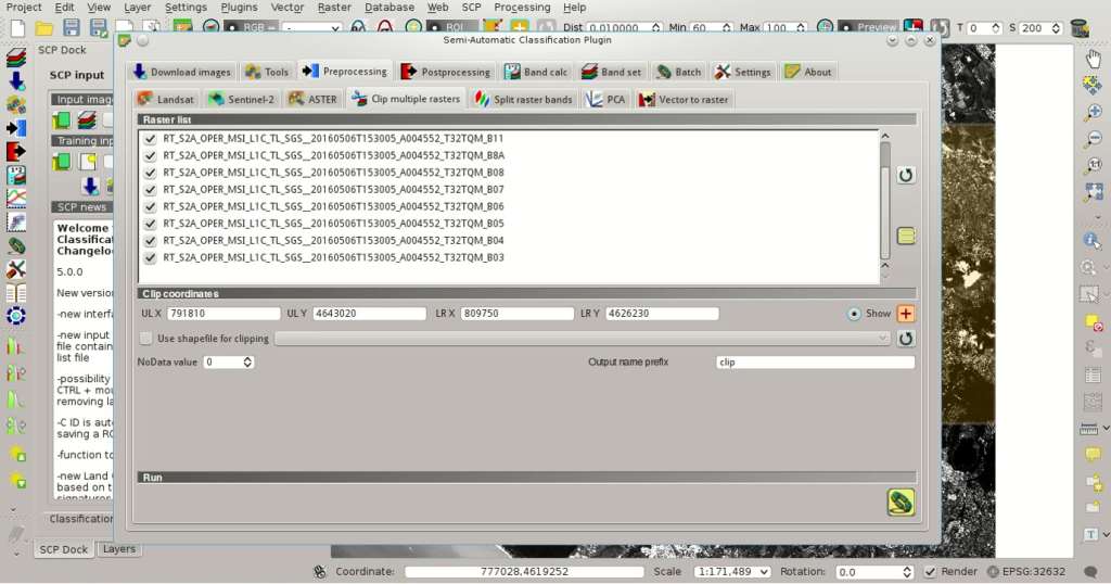
Clip area

Click the button and select a directory (e.g. clip) where clipped bands are saved (with the file name prefix defined in Output name prefix). When the process is completed, clipped rasters are loaded and displayed. We can remove the bands whose names start with RT_ from QGIS layers.

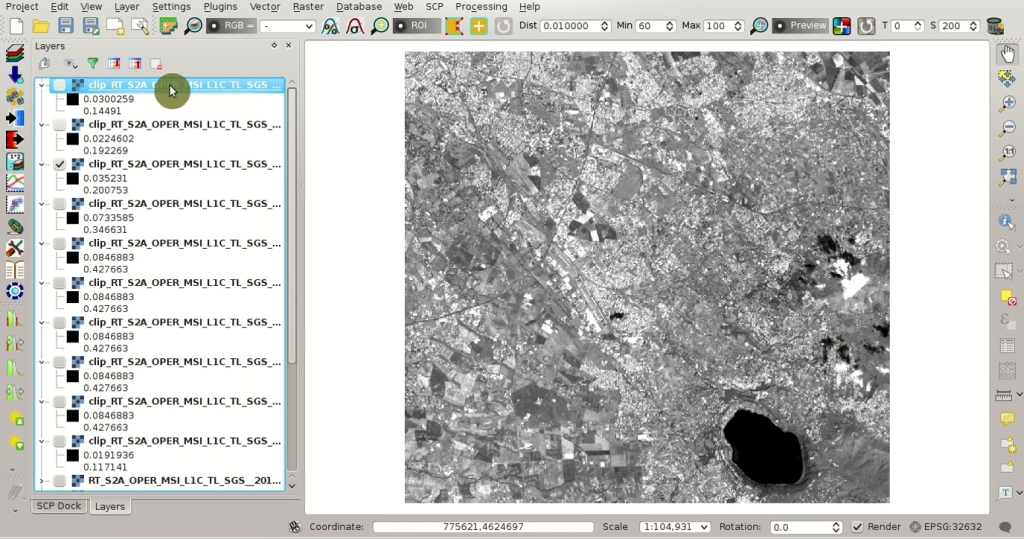
Clipped bands

4.2.1.4. Create the Band Set ¶

Now we need to define the Band set which is the input image for SCP. Open the tab Band set clicking the button in the SCP menu, or the SCP Tools, or the SCP dock.

Click the button to refresh the layer list, and check all the clipped bands; then click to add selected rasters to the Band set. In the table Band set definition order the band names in ascending order (click to sort bands by name automatically), then highlight band 8A (i.e. single click on band name in the table) and use the buttons or to place this band at number 8. Finally, select Sentinel-2 from the list Quick wavelength settings, in order to set automatically the Center wavelength of each band and the Wavelength unit (required for spectral signature calculation).

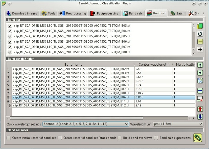
Definition of a band set

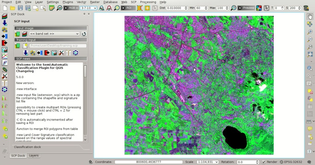
You can notice that the item << band set >> is selected as Input image in the SCP dock.

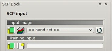
Band set

4.2.1.5. Create the ROIs ¶

In order to collect ROIs we need to Create the Training Input File as described in Tutorial 1: Your First Land Cover Classification (in the SCP dock click the button and define a file name). The Training input stores the ROIs and the Spectral Signature thereof.

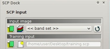
Definition of Training input in SCP

We are going to create several ROIs using the Macroclass IDs defined in the following table (see Classes and Macroclasses).

Macroclasses

Macroclass name	Macroclass ID
Water	1
Built-up	2
Vegetation	3
Bare soil	4

In this phase we are creating the database of spectral signatures used to identify land cover classes (the ones defined as macroclasses). However, these macroclasses are composed of several materials having different spectral signatures; in order to achieve good classification results we should separate spectral signatures of different materials, even if belonging to the same macroclass. Thus, we are going to create several ROIs for each macroclass (setting the same MC ID, but assigning a different C ID to every ROI).

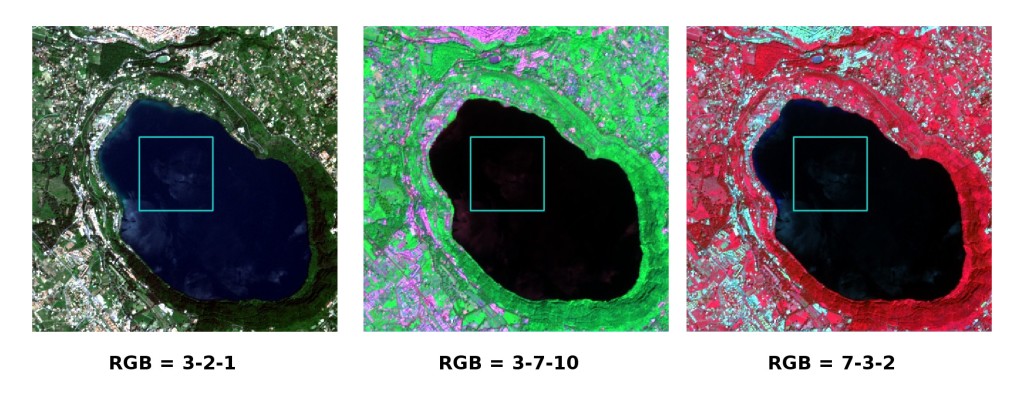
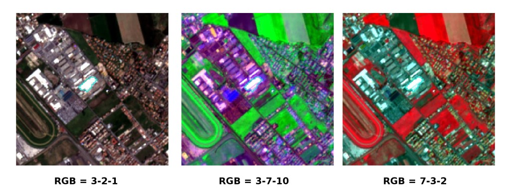
In the list RGB= of Working toolbar select 3-2-1 to display a natural color image (see ref:color_composite_definition and Sentinel-2 Satellite). After a few seconds, the Color Composite will be displayed. We can see that urban areas are white and vegetation is green.

TIP : If a Band set is defined, a temporary virtual raster (named band_set.vrt) is created automatically, which allows for the display of Color Composite. In order to speed up the visualization, you can show only the virtual raster and hide all the layers in the QGIS Layers.

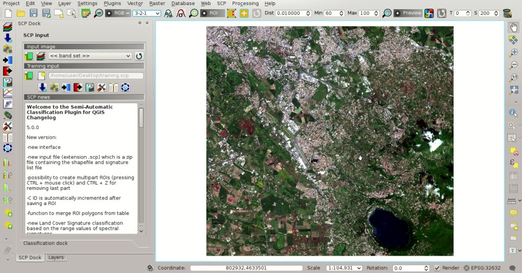
Color composite RGB = 3-2-1

Now in the list RGB= of the Working toolbar type 3-7-10 (you can also use the tool RGB list). Using this color composite, urban areas are purple and vegetation is green. You can notice that this color composite RGB = 3-7-10 highlights roads more than natural color (RGB = 3-2-1). Also, you can see that there are clouds in the right part of the image.

Color composite RGB = 3-7-10

Now create the ROIs following the same steps described in Create the ROIs of Tutorial 1: Your First Land Cover Classification. After clicking the button in the Working toolbar you should notice that the cursor in the map displays a value changing over the image. This is the NDVI value of the pixel beneath the cursor (NDVI is displayed because the function Display is checked in ROI creation). The NDVI value can be useful for identifying spectrally pure pixels, in fact vegetation has higher NDVI values than soil.

For instance, move the mouse over a vegetation area and left click to create a ROI when you see a local maximum value. This way, the created ROI and the spectral signature thereof will be particularly representative of healthy vegetation.

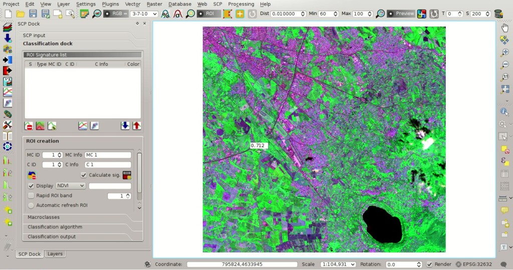
NDVI value of vegetation pixel displayed in the map

The color composite RGB = 7-3-2 is also useful for highlighting vegetation.

Create several ROIs (the more is the better). The region growing algorithm can create more homogeneous ROIs (i.e. standard deviation of spectral signature values is low) than manually drawn ones; the manual creation of ROIs can be useful in order to account for the spectral variability of classes (especially when using the algorithm Maximum Likelihood).

In general, you should create one ROI for each color that you can distinguish in the image. Therefore, change the color composite in order to identify the different types of land cover.

TIP : Change frequently the Color Composite in order to clearly identify the materials at the ground; use the mouse wheel on the list RGB= of the Working toolbar for changing the color composite rapidly; also use the buttons and for better displaying the Input image (i.e. image stretching).

A few examples of ROIs are illustrated in the following figures.

Water ROI: lake

Built-up ROI: large buildings

Built-up ROI: road

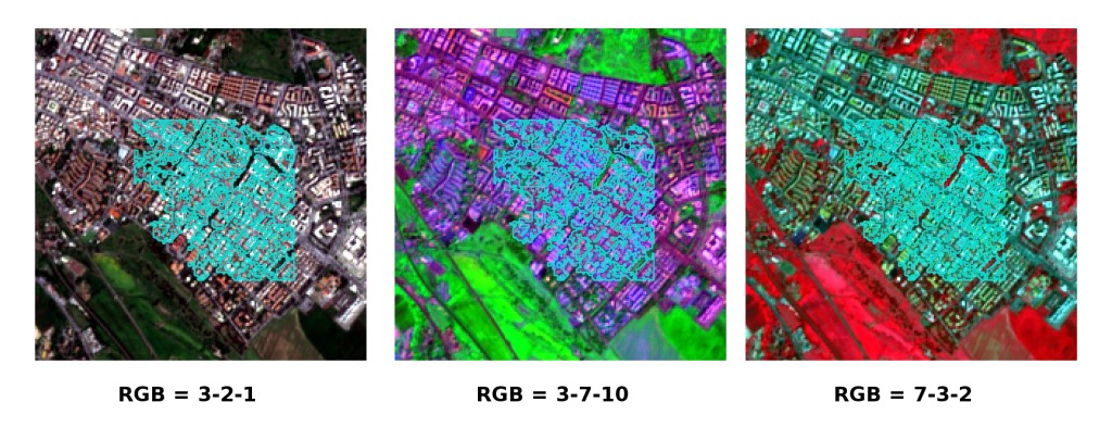
Built-up ROI: buildings and narrow roads

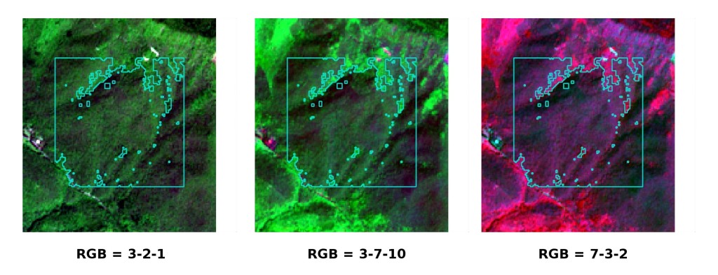
Vegetation ROI: deciduous trees

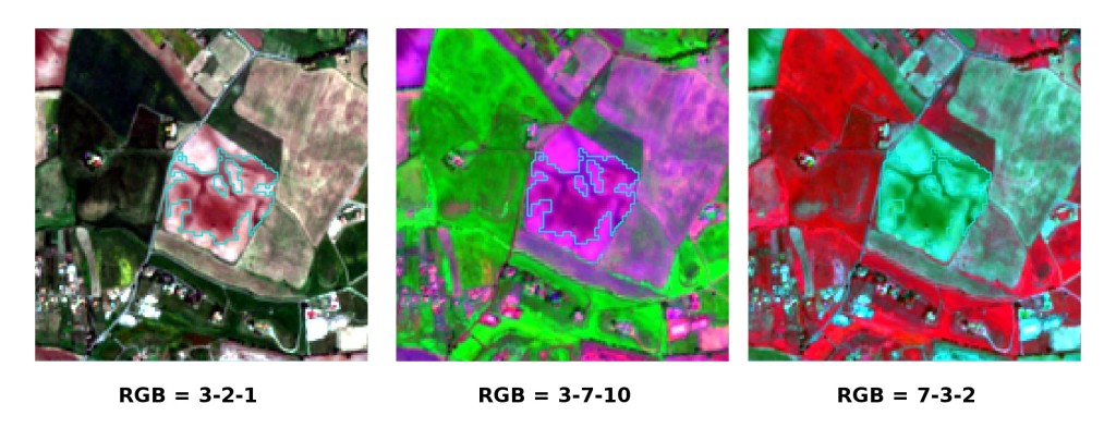
Vegetation ROI: crop

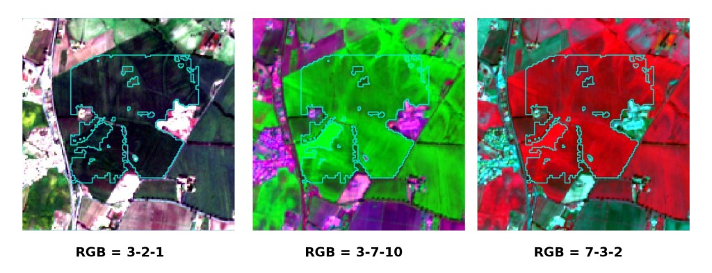
Bare soil ROI: uncultivated land

It is worth mentioning that you can show or hide the temporary ROI clicking the button ROI in Working toolbar.

TIP : Install the plugin QuickMapServices in QGIS, and add a map (e.g. OpenStreetMap) in order to facilitate the identification of ROIs using high resolution data.

We can also try to mask clouds in the image, creating ROIs of clouds and assigning the special MC ID = 0 (which is an ID used for labelling intentionally unclassified pixels) and a different C ID. In fact spectral signatures with the MC ID = 0 are normally used in the classification, but every pixel assigned to these spectral signatures is labelled unclassified in the classification result. Therefore, this is a simple way for masking particular spectral signatures such as clouds (of course there are more advanced methods for masking clouds that will be discussed in other tutorials).

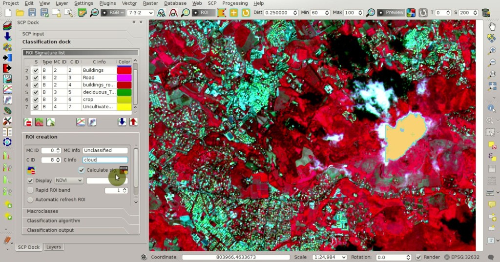
Example of ROI for clouds

4.2.1.6. Create a Classification Preview ¶

As pointed out in Tutorial 1: Your First Land Cover Classification, previews are temporary classifications that are useful for assessing the effects of spectral signatures during the ROI collection.

Set the colors of the spectral signatures in the ROI Signature list; then, in the Classification algorithm select the classification algorithm Maximum Likelihood. In Classification preview set Size = 500; click the button and then left click a point of the image in the map.

The classification preview is displayed in the map.

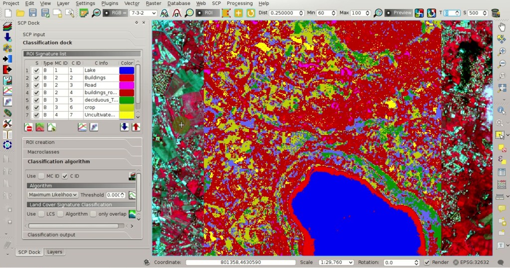
Example of preview using C IDs

In order to create a classification preview using Macroclass IDs check the option MC ID in the tab Classification algorithm of the SCP dock. In the tab Macroclasses of the SCP dock change the colors of MC ID (in the table Macroclasses double click the color of each macroclass to choose a representative color).

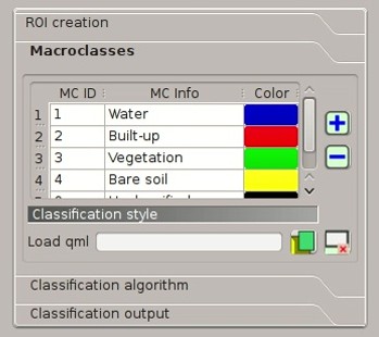
COlors of MC IDs

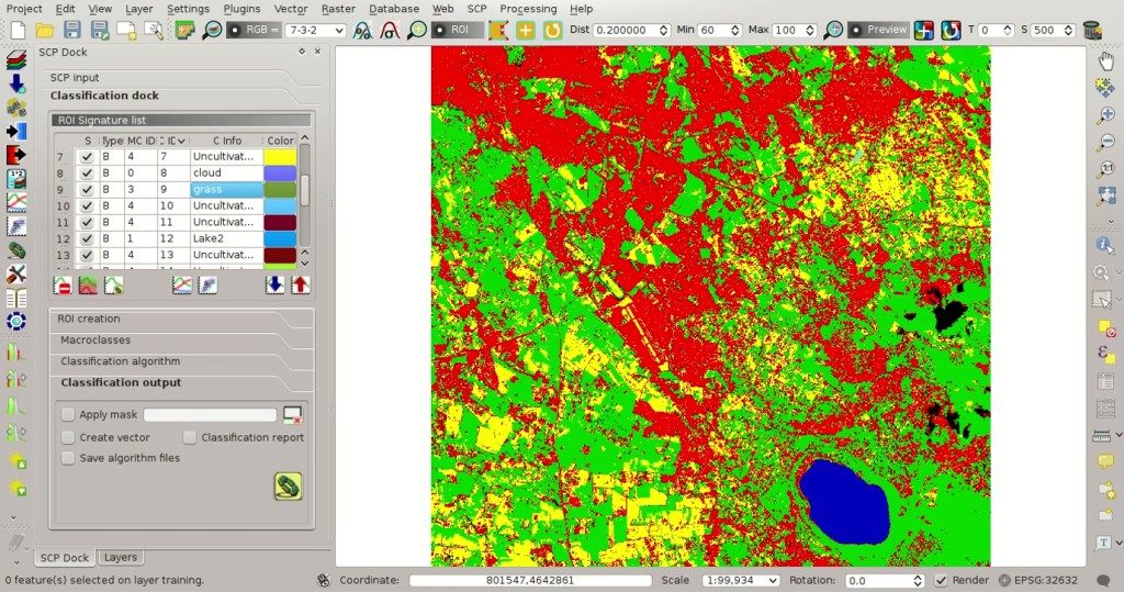
Now click the button in the Working toolbar to calculate a new preview at the same area of the previous one. In the following figure you can notice that there are fewer classes (only the MC ID) than the previous preview; also, clouds are unclassified (black pixels).

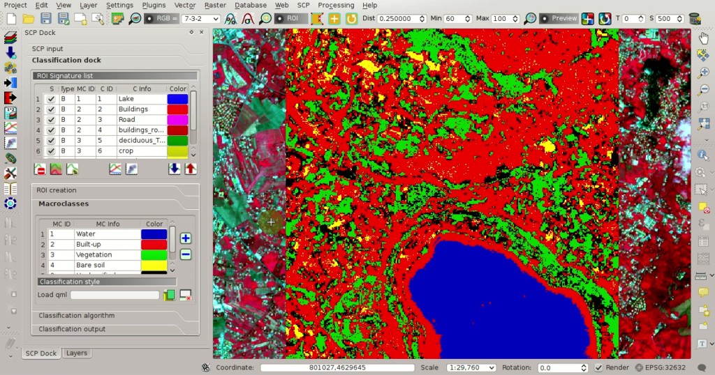
TIP : In the Working toolbar click the button Preview to easily show or hide the classification previews, and the button RGB= to show or hide the Input image.

Example of preview using MC IDs

4.2.1.7. Assess Spectral Signatures ¶

Spectral signatures are used by Classification Algorithms for labelling image pixels. Different materials may have similar spectral signatures (especially considering multispectral images) such as built-up and soil. If spectral signatures used for classification are too similar, pixels could be misclassified because the algorithm is unable to discriminate correctly those signatures. Thus, it is useful to assess the Spectral Distance of signatures to find similar spectral signatures that must be removed. Of course the concept of distance vary according to the algorithm used for classification.

One can simply assess spectral signature similarity by displaying a signature plot. In order to display the signature plot, in the ROI Signature list highlight two or more spectral signatures (with click in the table), then click the button . The Spectral Signature Plot is displayed in a new window. Move ans zoom inside the Plot to see if signatures are similar (i.e. very close). We can see in the following figure a signature plot of different materials.

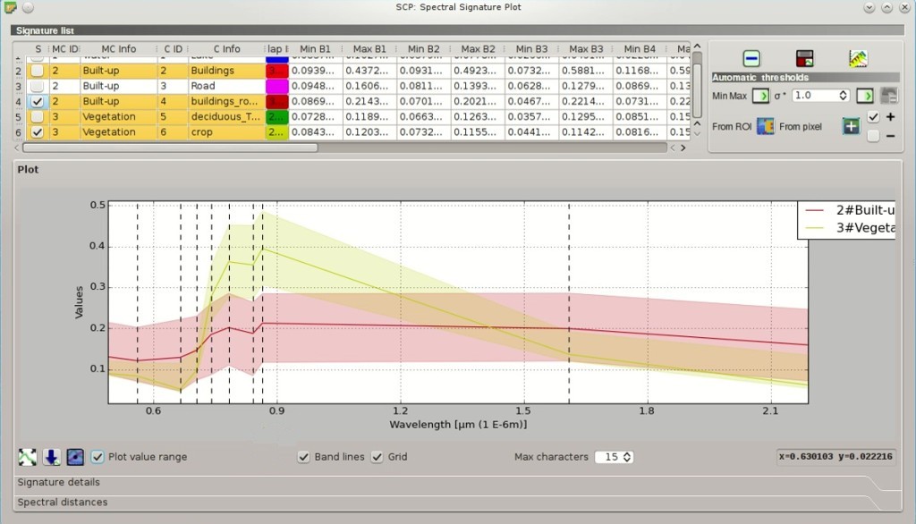
Spectral plot

In the plot we can see the line of each signature (with the color defined in the ROI Signature list), and the spectral range (minimum and maximum) of each band (i.e. the semi-transparent area colored like the signature line). The larger is the semi-transparent area of a signature, the higher is the standard deviation, and therefore the heterogeneity of pixels that composed that signature. Spectral signature values are displayed in the Signature details.

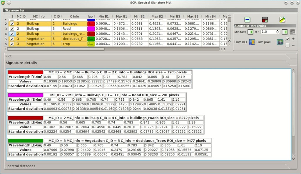
Spectral signature values

Additionally, we can calculate the spectral distances of signatures (for more information see Spectral Distance). Highlight two or more spectral signatures with click in the table Plot Signature list, then click the button ; distances will be calculated for each pair of signatures. Now open the tab Spectral distances; we can notice that similarity between signatures vary according to considered algorithm.

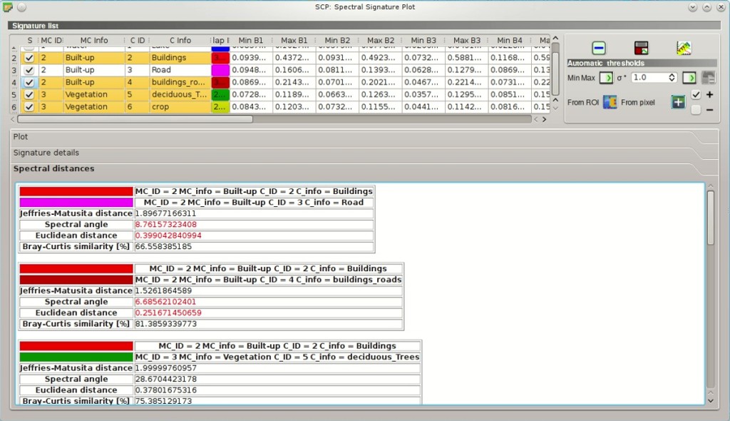
Spectral distances

For instance, two signatures can be very similar Spectral Angle Mapping (very low Spectral Angle), but quite distant for the Maximum Likelihood (Jeffries-Matusita Distance value near 2). The similarity of signatures is affected by the similarity of materials (in relation to the number of spectral bands available in the Input image); also, the way we create ROIs influences the signatures.

4.2.1.8. Create the Classification Output ¶

Repeat iteratively the phases Create the ROIs, Create a Classification Preview, and Assess Spectral Signatures until the classification previews show good results.

To start the classification of the entire image, open the tab Classification output, click the button and define the name of the classification output.

TIP : Set the Available RAM (MB) in RAM settings, in order to reduce the computational time; the recommended value is half of the system RAM.

If Play sound when finished is checked in Classification process settings, a sound is played when the process is finished.

Classification

It is worth mentioning that SCP provides other tools and techniques that can improve the classification results, which are described in Thematic Tutorials.