3. Breve Introduzione al Telerilevamento (Remote Sensing)

3.1. Definizioni Base

This chapter provides basic definitions about GIS and remote sensing. For other useful resources see Free and valuable resources about remote sensing and GIS.

3.1.1. GIS definizione

Esistono diverse definizioni di ** ** GIS (Geographic Information Systems), che non è semplicemente un programma. In generale, i GIS sono sistemi che consentono l’utilizzo di informazioni geografiche (dati che hanno coordinate spaziali). In particolare, i GIS permettono la visualizzazione, l’interrogazione, il calcolo e l’analisi dei dati spaziali, che principalmente si distinguono in raster e vettori. I Vettori sono oggetti di tipo puntuale o lineare o poligonale, e ogni oggetto può avere uno o più valori di attributi; un raster è una griglia (o immagine) in cui ogni cella ha un valore di attributo (Fisher Unwin, 2005). Le applicazioni GIS utilizzano immagini raster che sono derivati da telerilevamento.

3.1.2. Telerilevamento definizione

Una definizione generale di ** ** Remote Sensing è: “la scienza e la tecnologia con la quale le caratteristiche degli oggetti di interesse possono essere identificate, misurate e analizzate senza contatto diretto” (JARS, 1993).

Solitamente, il telerilevamento misura l’energia che viene emanata dalla superficie terrestre. Se la sorgente dell’energia misurata è il sole, allora si chiama ** telerilevamento passivo **, e il risultato di questa misurazione può essere un’immagine digitale (Richards e Jia, 2006). Se l’energia misurata non viene emessa dal Sole, ma da un sensore artificiale allora è definito come ** telerilevamento attivo **, come i radar stellite che operano nel campo delle microonde (Richards e Jia, 2006) radar.

Lo spettro elettromagnetico è “il sistema che classifica, secondo la lunghezza d’onda, tutta l’energia (da breve a lungo cosmica radio) che si muove, armonicamente, alla velocità costante di luce” (NASA, 2013). I sensori passivi misurano l’energia dalle regioni ottiche dello spettro elettromagnetico: visibile, vicino infrarosso (NIR), infrarosso a onde corte (SWIR) e infrarosso termico (TM) (vedi Figura: ref: figEM).

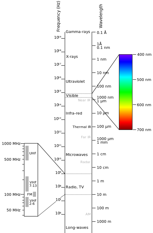
Spettro-Elettromagnetico

by Victor Blacus (SVG version of File:Electromagnetic-Spectrum.png)

[CC-BY-SA-3.0 (http://creativecommons.org/licenses/by-sa/3.0)]

via Wikimedia Commons

http://commons.wikimedia.org/wiki/File%3AElectromagnetic-Spectrum.svg

L’interazione tra energia solare e materiali dipende dalla lunghezza d’onda; energia solare va dal Sole alla Terra e poi al sensore. Lungo questo percorso, **l’energia solare ** è (NASA, 2013):

• ** Trasmesso ** - L’energia passa da un mezzo a un altro venendo rifratta come determinato dall’indice di rifrazione dei due mezzi in questione.

• ** Assorbita ** - L’energia è assorbita da un oggetto attraverso reazioni di elettroni o molecolari.

• ** Riflessa ** - L’energia viene restituito invariato con un angolo di incidenza uguale all’angolo di riflessione. La riflettanza è il rapporto tra l’energia riflessa a quella incidente su un corpo. La lunghezza d’onda riflessa (non assorbita) determina il colore di un oggetto.

• Dispersa - La direzione di propagazione dell’energia è cambia in modo casuale. Rayleigh e Mie sono i due più importanti tipi di dispersione in atmosfera.

• ** Emessa** - In realtà, l’energia viene prima assorbita, poi ri-emessa, di solito a lunghezze d’onda maggiori. L’oggetto si riscalda.

3.1.3. Sensori

** I sensori ** possono essere a bordo di aerei o a bordo di satelliti, per misurare la radiazione elettromagnetica a intervalli specifici (generalmente chiamati bande). Come risultato, le misure sono quantizzate e convertite in un’immagine digitale, in cui ogni elemento di immagine (pixel) ha un valore discreto in unità di Digital Number (DN) (NASA, 2013). Le immagini risultanti hanno caratteristiche diverse (risoluzioni) a seconda del sensore. Ci sono diversi tipi di risoluzioni:

• La risoluzione spaziale, di solito misurata in dimensione dei pixel, “è il potere di risoluzione di uno strumento necessario per la discriminazione delle caratteristiche e si basa sulla dimensione del sensore, distanza focale, e altitudine del sensore ” (NASA, 2013); risoluzione spaziale è indicata anche come risoluzione geometrica o IFOV;

• Risoluzione spettrale , è il numero e la posizione nello spettro elettromagnetico (definito da due lunghezze d’onda) delle bande spettrali (NASA, 2013) in sensori multispettrali, per ogni banda corrisponde un’immagine;

• ** Risoluzione radiometrica **, solitamente misurata in bit (cifre binarie), è la gamma di valori di luminosità disponibili, che nell’immagine corrispondono alla portata massima dei DN; per esempio, un’immagine con risoluzione di 8 bit dispone di 256 livelli di luminosità (Richards e Jia, 2006);

• Per i sensori satellitari, si misura anche la risoluzione temporale, che è il tempo necessario per rivisitare la stessa area della Terra (NASA, 2013).

3.1.4. Radianza e Riflettanza

I sensori misurano la radianza, che corrisponde alla luminosità in una certa direzione verso il sensore; inoltre è utile definire la riflettanza come il rapporto tra l’energia riflessa e l’energia totale.

3.1.5. Firma Spettrale

The spectral signature is the reflectance as a function of wavelength (see Figure : guilabel: curva di riflettanza spettrale di quattro diversi oggetti); each material has a unique signature, therefore it can be used for material classification (NASA, 2013).

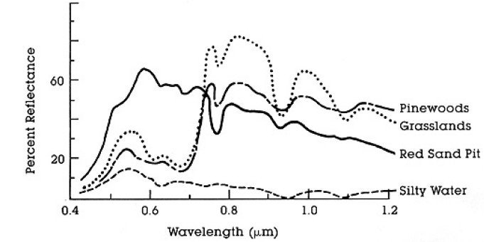
: guilabel: curva di riflettanza spettrale di quattro diversi oggetti

(NASA, 2013)`

3.1.6. Satellite Landsat

Landsat è un insieme di satelliti multispettrali sviluppato dalla NASA (National Aeronautics and Space Administration degli Stati Uniti), sin dagli inizi del 1970.

Le immagini Landsat sono molto utilizzate per la ricerca ambientale. Le risoluzioni dei sensori Landsat 4 e Landsat 5 sono riportate nella seguente tabella (da http://landsat.usgs.gov/band_designations_landsat_satellites.php); Inoltre, risoluzione temporale Landsat è di 16 giorni (NASA, 2013).

Landsat 4 and Landsat 5 Bands

Bande Landsat 4, Landsat 5	Lunghezza d’onda [micrometri]	Risoluzione [metri]
Banda 1 - Blu	0.45 - 0.52	30
Banda 2 - Verde	0.52 - 0.60	30
Banda 3 - Rosso	0.63 - 0.69	30
Banda 4 - Vicino Infrarosso (NIR)	0.76 - 0.90	30
Banda 5 - Onde corte Infrarosso (SWIR)	1.55 - 1.75	30
Banda 6 - Infrarosso termico (TI)	10.40 - 12.50	120 (ricampionata a 30)
Banda 7 - SWIR	2.08 - 2.35	30

Le risoluzioni del sensore Landsat 7 sono riportate nella seguente tabella (da http://landsat.usgs.gov/band_designations_landsat_satellites.php); Inoltre, la risoluzione temporale Landsat è di 16 giorni (NASA, 2013).

Landsat 7 Bands

Landsat 7 Bands	Lunghezza d’onda [micrometri]	Risoluzione [metri]
Banda 1 - Blu	0.45 - 0.52	30
Banda 2 - Verde	0.52 - 0.60	30
Banda 3 - Rosso	0.63 - 0.69	30
Banda 4 - Vicino Infrarosso (NIR)	0.77 - 0.90	30
Banda 5 - Onde corte Infrarosso (SWIR)	1.57 - 1.75	30
Banda 6 - Infrarosso termico (TI)	10.40 - 12.50	60 (ricampionate a 30)
Banda 7 - SWIR	2.09 - 2.35	30
Band 8 - Panchromatica	0.52 - 0.90	15

Le risoluzioni del sensore Landsat 8 sono riportate nella seguente tabella (da http://landsat.usgs.gov/band_designations_landsat_satellites.php); Inoltre, la risoluzione temporale Landsat è di 16 giorni (NASA, 2013)

Landsat 8 Bands

Bande Landsat 8	Lunghezza d’onda [micrometri]	Risoluzione [metri]
Banda 1 - Aerosol costiero	0.43 - 0.45	30
Band 2 - Blue	0.45 - 0.51	30
Banda 3 - Verde	0.53 - 0.59	30
Banda 4 - Rosso	0.64 - 0.67	30
Band 5 - Infrarosso Vicino (NIR)	0.85 - 0.88	30
Band 6 - SWIR 1	1.57 - 1.65	30
Band 7 - SWIR 2	2.11 - 2.29	30
Band 8 - Panchromatica	0.50 - 0.68	15
Band 9 - Cirro	1.36 - 1.38	30
Band 10 - Infrarosso Termico (TIRS) 1	10.60 - 11.19	100 (resampled to 30)
Band 11 - Infrarosso Termico (TIRS) 2	11.50 - 12.51	100 (resampled to 30)

A vast archive of images is freely available from the U.S. Geological Survey . For more information about how to freely download Landsat images read this .

Images are identified with the paths and rows of the WRS (Worldwide Reference System for Landsat ).

3.1.7. Sentinel-2 Satellite

Sentinel-2 è un satellite multispettrale sviluppato dall’Agenzia Spaziale Europea (ESA) nel quadro di Copernicus land monitoring services. Sentinel-2 acquisisce 13 bande spettrali con la risoluzione spaziale di 10m, 20m e 60m a seconda della fascia, come illustrato nella seguente tabella (ESA, 2015).

Sentinel-2 Bands

Sentinel-2 Bande	Central Wavelength [micrometers]	Risoluzione [metri]
Banda 1 - Aerosol costiero	0.443	60
Band 2 - Blue	0.490	10
Banda 3 - Verde	0.560	10
Banda 4 - Rosso	0.665	10
Band 5 - Vegetation Red Edge	0.705	20
Band 6 - Vegetation Red Edge	0.740	20
Band 7 - Vegetation Red Edge	0.783	20
Band 8 - NIR	0.842	10
Band 8A - Vegetation Red Edge	0.865	20
Band 9 - Water vapour	0.945	60
Band 10 - SWIR - Cirrus	1.375	60
Band 11 - SWIR	1.610	20
Band 12 - SWIR	2.190	20

Le immagini Sentinel-2 sono liberamente disponibili sul sito web dell’ESA https://scihub.esa.int/dhus/.

3.1.8. ASTER Satellite

The ASTER (Advanced Spaceborne Thermal Emission and Reflection Radiometer) satellite was launched in 1999 by a collaboration between the Japanese Ministry of International Trade and Industry (MITI) and the NASA. ASTER has 14 bands whose spatial resolution varies with wavelength: 15m in the visible and near-infrared, 30m in the short wave infrared, and 90m in the thermal infrared (USGS, 2015). ASTER bands are illustrated in the following table (due to a sensor failure SWIR data acquired since April 1, 2008 is not available ). An additional band 3B (backwardlooking near-infrared) provides stereo coverage.

ASTER Bands

ASTER Bands	Lunghezza d’onda [micrometri]	Risoluzione [metri]
Band 1 - Green	0.52 - 0.60	15
Band 2 - Red	0.63 - 0.69	15
Band 3N - Near Infrared (NIR)	0.78 - 0.86	15
Band 4 - SWIR 1	1.60 - 1.70	30
Band 5 - SWIR 2	2.145 - 2.185	30
Band 6 - SWIR 3	2.185 - 2.225	30
Band 7 - SWIR 4	2.235 - 2.285	30
Band 8 - SWIR 5	2.295 - 2.365	30
Band 9 - SWIR 6	2.360 - 2.430	30
Band 10 - TIR 1	8.125 - 8.475	90
Band 11 - TIR 2	8.475 - 8.825	90
Band 12 - TIR 3	8.925 - 9.275	90
Band 13 - TIR 4	10.25 - 10.95	90
Band 14 - TIR 5	10.95 - 11.65	90

3.1.9. MODIS Products

The MODIS (Moderate Resolution Imaging Spectroradiometer) is an instrument operating on the Terra and Aqua satellites launched by NASA in 1999 and 2002 respectively. Its temporal resolutions allows for viewing the entire Earth surface every one to two days, with a swath width of 2,330. Its sensors measure 36 spectral bands at three spatial resolutions: 250m, 500m, and 1,000m (see https://lpdaac.usgs.gov/dataset_discovery/modis).

Several products are available, such as surface reflectance and vegetation indices. In this manual we are considering the surface reflectance bands available at 250m and 500m spatial resolution (Vermote, Roger, & Ray, 2015).

MODIS Bands

MODIS Bands	Lunghezza d’onda [micrometri]	Risoluzione [metri]
Band 1 - Red	0.62 - 0.67	250 - 500
Band 2 - Near Infrared (NIR)	0.841 - 0.876	250 - 500
Band 3 - Blue	0.459 - 0.479	500
Band 4 - Green	0.545 - 0.565	500
Band 5 - SWIR 1	1.230 - 1.250	500
Band 6 - SWIR 2	1.628 - 1.652	500
Band 7 - SWIR 3	2.105 - 2.155	500

The following products (Version 6, see https://lpdaac.usgs.gov/dataset_discovery/modis/modis_products_table) are available for download (Vermote, Roger, & Ray, 2015):

• MOD09GQ: daily reflectance at 250m spatial resolution from Terra MODIS;
• MYD09GQ: daily reflectance at 250m spatial resolution from Aqua MODIS;
• MOD09GA: daily reflectance at 500m spatial resolution from Terra MODIS;
• MYD09GA: daily reflectance at 500m spatial resolution from Aqua MODIS;
• MOD09Q1: reflectance at 250m spatial resolution, which is a composite of MOD09GQ (each pixel contains the best possible observation during an 8-day period);
• MYD09Q1: reflectance at 250m spatial resolution, which is a composite of MYD09GQ (each pixel contains the best possible observation during an 8-day period);
• MOD09A1: reflectance at 250m spatial resolution, which is a composite of MOD09GA (each pixel contains the best possible observation during an 8-day period);
• MYD09A1: reflectance at 250m spatial resolution, which is a composite of MYD09GA (each pixel contains the best possible observation during an 8-day period);

3.1.10. Colore Composito

Spesso, una combinazione viene creata da tre immagini monocromatiche individuali, in cui a ciascuna è assegnato un dato colore; questa è definita ** color composite ** ed è utile per la fotointerpretazione (NASA, 2013). Le color composite sono di solito espresse come:

“R G B = Br Bg Bb”

where:

• R sta per rosso;

• G sta per verde;

• B sta per Blue;

• Br è il numero di banda associato al colore rosso;

• Bg è il numero di banda associato al colore verde;

• Bb è il numero di banda associato al colore blu.

The following Figure : guilabel: Colore composito di un immagine Landsat8 shows a color composite “R G B = 4 3 2” of a Landsat 8 image (for Landsat 7 the same color composite is R G B = 3 2 1; for Sentinel-2 is R G B = 4 3 2) and a color composite “R G B = 5 4 3” (for Landsat 7 the same color composite is R G B = 4 3 2; for Sentinel-2 is R G B = 8 4 3). The composite “R G B = 5 4 3” is useful for the interpretation of the image because vegetation pixels appear red (healthy vegetation reflects a large part of the incident light in the near-infrared wavelength, resulting in higher reflectance values for band 5, thus higher values for the associated color red).

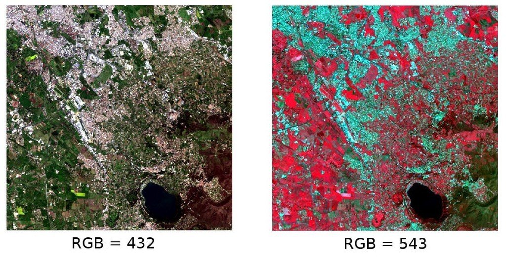
: guilabel: Colore composito di un immagine Landsat8

I dati disponibili da U.S. Geological Survey

3.1.11. Principal Component Analysis

Principal Component Analysis (PCA) is a method for reducing the dimensions of measured variables (bands) to the principal components (JARS, 1993).

Th principal component transformation provides a new set of bands (principal components) having the following characteristic: principal components are uncorrelated; each component has variance less than the previous component. Therefore, this is an efficient method for extracting information and data compression (Ready and Wintz, 1973).

Given an image with N spectral bands, the principal components are obtained by matrix calculation (Ready and Wintz, 1973; Richards and Jia, 2006):

\[Y = D^t X\]

where:

• \(Y\) = vector of principal components
• \(D\) = matrix of eigenvectors of the covariance matrix \(C_x\) in X space
• \(t\) denotes vector transpose

And \(X\) is calculated as:

\[X = P - M\]

• \(P\) = vector of spectral values associated with each pixel
• \(M\) = vector of the mean associated with each band

Thus, the mean of \(X\) associated with each band is 0. \(D\) is formed by the eigenvectors (of the covariance matrix \(C_x\)) ordered as the eigenvalues from maximum to minimum, in order to have the maximum variance in the first component. This way, the principal components are uncorrelated and each component has variance less than the previous component(Ready and Wintz, 1973).

Usually the first two components contain more than the 90% of the variance. For example, the first principal components can be displayed in a Colore Composito for highlighting Land Cover classes, or used as input for Supervised Classification.

3.1.12. Pan-sharpening

Pan-sharpening is the combination of the spectral information of multispectral bands (MS), which have lower spatial resolution (for Landsat bands, spatial resolution is 30m), with the spatial resolution of a panchromatic band (PAN), which for Landsat 7 and 8 it is 15m. The result is a multispectral image with the spatial resolution of the panchromatic band (e.g. 15m). In SCP, a Brovey Transform is applied, where the pan-sharpened values of each multispectral band are calculated as (Johnson, Tateishi and Hoan, 2012):

\[MSpan = MS * PAN / I\]

dove:: I è intensità, che è una funzione di bande multispettrali.

The following weights for I are defined, basing on several tests performed using the SCP. For Landsat 8, Intensity is calculated as:

\[I = (0.42 * Blue + 0.98 * Green + 0.6 * Red ) / 2\]

Per Landsat 7, l’ Intensità è così calcolata:

\[I = (0.42 * Blue + 0.98 * Green + 0.6 * Red + NIR) / 3\]

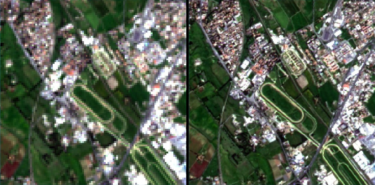
Esempio di pan-sharpening di un’immagine Landsat 8. Sinistra, bande multispettrali originali (30m); a destra, pan-sharpened (15m)

I dati disponibili da U.S. Geological Survey

3.1.13. Spectral Indices

Spectral indices are operations between spectral bands that are useful for extracting information such as vegetation cover (JARS, 1993). One of the most popular spectral indices is the Normalized Difference Vegetation Index (NDVI), defined as (JARS, 1993):

\[NDVI = ( NIR - Red ) / ( NIR + Red )\]

NDVI values range from -1 to 1. Dense and healthy vegetation show higher values, while non-vegetated areas show low NDVI values.

Another index is the Enhanced Vegetation Index (EVI) which attempts to account for atmospheric effects such as path radiance calculating the difference between the blue and the red bands (Didan,et al., 2015). EVI is defined as:

\[EVI = G ( NIR - Red ) / ( NIR + C_1 Red - C_2 Blue + L)\]

where: \(G\) is a scaling factor, \(C_1\) and \(C_2\) are coefficients for the atmospheric effects, and \(L\) is a factor for accounting the differential NIR and Red radiant transfer through the canopy. Typical coefficient values are: \(G = 2.5\), \(L = 1\), \(C_1 = 6\), \(C_2 = 7.5\) (Didan,et al., 2015).

3.2. Supervised Classification Definizioni

Questo capitolo fornisce le definizioni di base riguardoa alla supervised classifications.

3.2.1. Land Cover

Land cover è il materiale a terra, come il suolo, la vegetazione, l’acqua, asfalto, ecc (Fisher e Unwin, 2005). In base alle risoluzione del sensore, il numero e il tipo di classi di copertura del suolo che può possono essere identificata nell’immagine possono variare significativamente.

3.2.2. Supervised Classification

Una classificazione semiautomatica (supervised classification) è una tecnica di elaborazione di immagini che permette l’identificazione di materiali in un’immagine, in base alle loro firme spettrali. Ci sono diversi tipi di algoritmi di classificazione, ma lo scopo generale è quello di produrre una mappa tematica della copertura del suolo.

Il processamento di immagini e le analisi spaziali richiedono specifici software come il Semi-Automatic Classification Plugin per QGIS

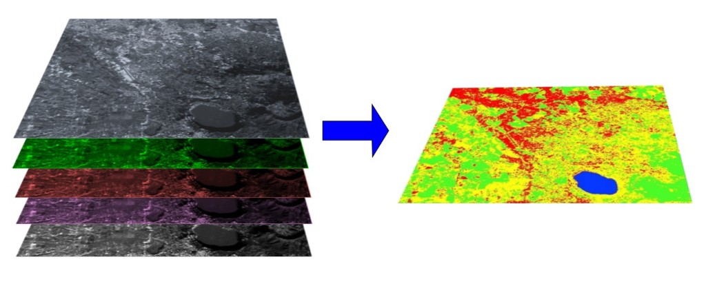
A multispectral image processed to produce a land cover classification

(Landsat image provided by USGS)

3.2.3. Training Areas

Di solito, le supervised classifications richiedono all’utente di selezionare uno o più regioni di interesse (ROI, o Training Areas) per ogni classe di copertura del suolo identificato nell’immagine. ** ROI** sono poligoni disegnati su aree omogenee dell’immagine che includoni pixel appartenenti alla stessa classe di copertura del suolo.

3.2.3.1. Region Growing Algorithm

The Region Growing Algorithm allows to select pixels similar to a seed one, considering the spectral similarity (i.e. spectral distance) of adjacent pixels. In SCP the Region Growing Algorithm is available for the training area creation. The parameter distance is related to the similarity of pixel values (the lower the value, the more similar are selected pixels) to the seed one (i.e. selected clicking on a pixel). An additional parameter is the maximum width, which is the side length of a square, centred at the seed pixel, which inscribes the training area (if all the pixels had the same value, the training area would be this square). The minimum size is used a constraint (for every single band), selecting at least the pixels that are more similar to the seed one until the number of selected pixels equals the minimum size.

In figure Region growing example the central pixel is used as seed (image a) for the region growing of one band (image b) with the parameter spectral distance = 0.1; similar pixels are selected to create the training area (image c and image d).

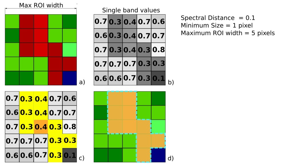
Region growing example

3.2.4. Classi e Macroclassi

Land cover classes are identified with an arbitrary ID code (i.e. Identifier). SCP allows for the definition of Macroclass ID (i.e. MC ID) and Class ID (i.e. C ID), which are the identification codes of land cover classes. A Macroclass is a group of ROIs having different Class ID, which is useful when one needs to classify materials that have different spectral signatures in the same land cover class. For instance, one can identify grass (e.g. ID class = 1 and Macroclass ID = 1 ) and trees (e.g. ID class = 2 and Macroclass ID = 1 ) as vegetation class (e.g. Macroclass ID = 1 ). Multiple Class IDs can be assigned to the same Macroclass ID, but the same Class ID cannot be assigned to multiple Macroclass IDs, as shown in the following table.

Example of Macroclasses

Macroclass name	Macroclass ID	Class name	Class ID
Vegetazione	1	Erba	1
Vegetazione	1	Alberi	2
Costruito	2	Buildings	3
Costruito	2	Roads	4

Pertanto, Le classi sono sottoinsiemi di un macroclasse come illustrato nella figura Macroclass esempio.

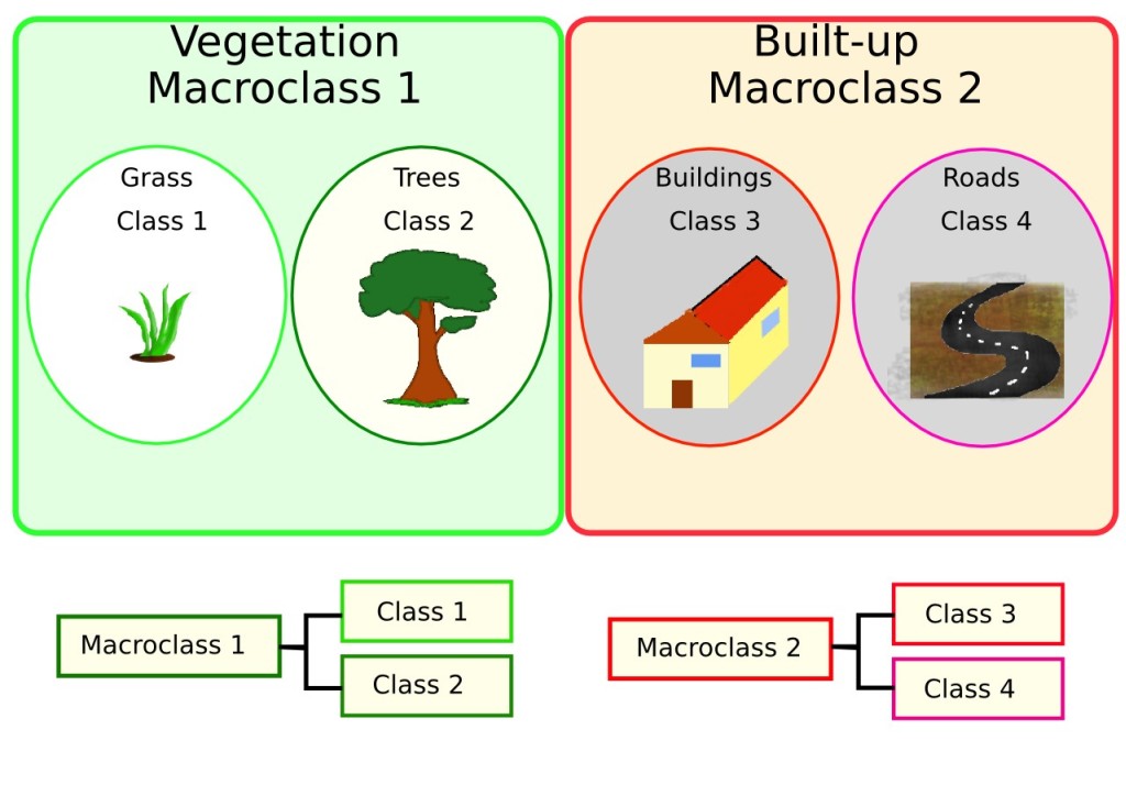
Macroclass esempio

Se per lo scopo dello studio non è richiesto l’uso della macroclasse, allora per tutte le ROIs può essere definito lo stesso ID di macroclasse (e.g. Macroclass ID = 1) e tutti i valori di macroclasse vengono ignorati durante la classificazione.

3.2.5. Classification Algorithms

The spectral signatures (spectral characteristics) of reference land cover classes are calculated considering the values of pixels under each ROI having the same Class ID (or Macroclass ID). Therefore, the classification algorithm classifies the whole image by comparing the spectral characteristics of each pixel to the spectral characteristics of reference land cover classes. SCP implements the following classification algorithms.

3.2.5.1. Minimum Distance

L’algoritmo Minimum Distance calcola la distanza euclidea: matematica: d (x, y) tra firme spettrali dei pixel dell’immagine e le firme spettrali delle ROI secondo la seguente equazione:

\[d(x, y) = \sqrt{ \sum_{i=1}^{n} (x_i - y_i)^2}\]

where:

• \(x\) = firma spettrale vettoriale di un pixel dell immagine;

• \(y\) = firma spettrale vettoriale della training area;

• \(n\) = numero di bande nell immagine.

Pertanto, la distanza è calcolata per ogni pixel nell’immagine, assegnandgli la classe della firma spettrale che gli è più vicina, secondo la seguente funzione discriminante (adattato da Richards e Jia, 2006):

\[x \in C_k \iff d(x, y_k) < d(x, y_j) \forall k \neq j\]

where:

• \(C_k\) = land cover class \(k\);

• \(y_k\) = firma spettrale della classe \(k\);

• \(y_j\) = firma spettrale della classe \(j\).

È possibile definire una soglia:math:T_i per escludere pixel sotto di questo valore dalla classificazione:

\[ \begin{align}\begin{aligned}x \in C_k \iff d(x, y_k) < d(x, y_j) \forall k \neq j\\and\\d(x, y_k) < T_i\end{aligned}\end{align} \]

3.2.5.2. Maximum Likelihood

L’algoritmo Maximum Likelihood calcola le distribuzioni di probabilità per le classi, relative al teorema di Bayes, stimando se un pixel appartiene a una classe di copertura del suolo. In particolare, le distribuzioni di probabilità per le classi si assumono la forma di modelli multivariati normali (Richards e Jia, 2006). Per utilizzare questo algoritmo, è necessario un numero sufficiente di pixel per ciascuna area di formazione consentendo il calcolo della matrice di covarianza. La funzione discriminante, descritta da Richards e Jia (2006), è calcolato per ogni pixel come

\[g_k(x) = \ln p(C_k) - \frac{1}{2} \ln | \Sigma_{k} | - \frac{1}{2} (x - y_k)^t \Sigma_{k}^{-1} (x - y_k)\]

where:

• \(C_k\) = land cover class \(k\);

• \(x\) = firma spettrale vettoriale di un pixel dell immagine;

• \(p(C_k)\) =probabilità che la classe sia corretta \(C_k\);

• \(| \Sigma_{k} |\) =determinante della matrice di covarianza dei dati nella classe:math:C_k;

• \(\Sigma_{k}^{-1}\) = inverso della matrice di covarianza;

• \(y_k\) = firma spettrale vettoriale della classe \(k\).

Dunque

\[x \in C_k \iff g_k(x) > g_j(x) \forall k \neq j\]

Maximum Likelihood example

inoltre, è possibile definire una soglia per la funzione discriminante per escludere pixel sotto di questo valore dalla classificazione. Considerando una soglia \(T_i\) la condizione di classificazione diventa:

\[ \begin{align}\begin{aligned}x \in C_k \iff g_k(x) > g_j(x) \forall k \neq j\\and\\g_k(x) > T_i\end{aligned}\end{align} \]

Maximum likelihood è una delle classificazioni supervisionate più comuni, ma il processo di classificazione può essere più lento di: ref: minimum_distance_algorithm.

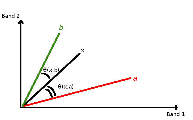
3.2.5.3. Spectral Angle Mapping

L’algoritmo Spectral Angle Mapping calcola l’angolo spettrale tra le firme spettrali dei pixel e le firme spettrali di riferimento. L’angolo spettrale: matematica: theta è definita come (Kruse et al., 1993):

\[\theta(x, y) = \cos^{-1} \left( \frac{ \sum_{i=1}^{n} x_i y_i } { \left( \sum_{i=1}^{n} x_i^2 \right)^\frac{1}{2} * \left( \sum_{i=1}^{n} y_i^2 \right)^\frac{1}{2} } \right)\]

Dove:

• \(x\) = firma spettrale vettoriale di un pixel dell immagine;

• \(y\) = firma spettrale vettoriale della training area;

• \(n\) = numero di bande nell immagine.

Perciò un pixel appartiene alla classe avente l’angolo più piccolo, cioè:

\[x \in C_k \iff \theta(x, y_k) < \theta(x, y_j) \forall k \neq j\]

where:

• \(C_k\) = land cover class \(k\);

• \(y_k\) = firma spettrale della classe \(k\);

• \(y_j\) = firma spettrale della classe \(j\).

Spectral Angle Mapping example

Per escludere pixel sotto questo valore dalla classificazione è possibile definire una soglia: matematica: T_i:

\[ \begin{align}\begin{aligned}x \in C_k \iff \theta(x, y_k) < \theta(x, y_j) \forall k \neq j\\and\\\theta(x, y_k) < T_i\end{aligned}\end{align} \]

Spectral Angle Mapping è largamente utilizzato, soprattutto con i dati iperspettrali.

3.2.5.4. Parallelepiped Classification

Parallelepiped classification is an algorithm that considers a range of values for each band, forming a multidimensional parallelepiped that defines a land cover class. A pixel is classified if the values thereof are inside a parallelepiped. One of the major drawbacks is that pixels whose signatures lie in the overlapping area of two or more parallelepipeds cannot be classified (Richards and Jia, 2006).

3.2.5.5. Land Cover Signature Classification

Land Cover Signature Classification is available in SCP (see Land Cover Signature Classification). This classification allows for the definition of spectral thresholds for each training input signature (a minimum value and a maximum value for each band). The thresholds of each training input signature define a spectral region belonging to a certain land cover class.

Spectral signatures of image pixels are compared to the training spectral signatures; a pixel belongs to class X if pixel spectral signature is completely contained in the spectral region defined by class X. In case of pixels falling inside overlapping regions or outside any spectral region, it is possible to use additional classification algorithms (i.e. Minimum Distance, Maximum Likelihood, Spectral Angle Mapping) considering the spectral characteristics of the original input signature.

In the following image, a scheme illustrates the Land Cover Signature Classification for a simple case of two spectral bands \(x\) and \(y\). User defined spectral regions define three classes (\(g_a\), \(g_b\), and \(g_c\)). Point \(p_1\) belongs to class \(g_a\) and point \(p_2\) belongs to class \(g_b\). However, point \(p_3\) is inside the spectral regions of both classes \(g_b\) and \(g_c\) (overlapping regions); in this case, point \(p_3\) will be unclassified or classified according to an additional classification algorithm. Point \(p_4\) is outside any spectral region, therefore it will be unclassified or classified according to an additional classification algorithm. Given that point \(p_4\) belongs to class \(g_c\), the spectral region thereof could be extended to include point \(p_4\) .

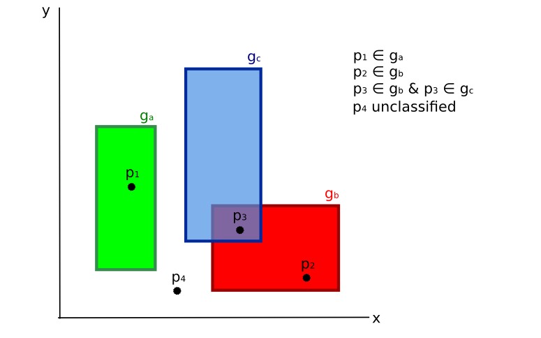
Land cover signature classification

This is similar to Parallelepiped Classification, with the exception that spectral regions are defined by user, and can be assigned independently for the upper and lower bounds. One can imagine spectral regions as the set of all the spectral signatures of pixels belonging to one class.

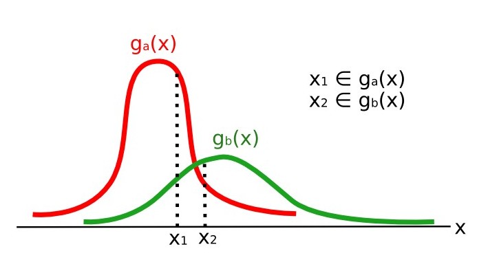
In figure Plot of spectral ranges the spectral ranges of three classes (\(g_a\), \(g_b\), and \(g_c\)) are displayed; the colored lines inside the ranges (i.e. semi-transparent area) represent the spectral signatures of pixels that defined the upper and lower bounds of the respective ranges. Pixel \(p_1\) (dotted line) belongs to class \(g_b\) because the spectral signature thereof is completely inside the range of class \(g_b\) (in the upper limit); pixel \(p_2\) (dashed line) is unclassified because the spectral signature does not fall completely inside any range; pixel \(p_3\) (dotted line) belongs to class \(g_a\).

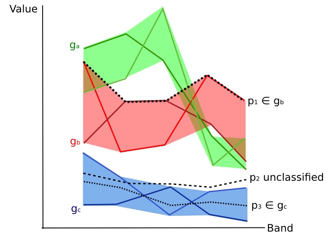
Plot of spectral ranges

It is worth noticing that these spectral thresholds can be applied to any spectral signature, regardless of spectral characteristics thereof; this function can be very useful for separating similar spectral signatures that differ only in one band, defining thresholds that include or exclude specific signatures. In fact, classes are correctly separated if the spectral ranges thereof are not overlapping at least in one band. Of course, even if spectral regions are overlapping, chances are that no pixel will fall inside the overlapping region and be misclassified; which is the upper (or lower) bound of a range do not imply the existence, in the image, of any spectral signature having the maximum (or minimum) range values for all the bands (for instance pixel \(p_1\) of figure Plot of spectral ranges could not exist).

One of the main benefit of the Land Cover Signature Classification is that it is possible to select pixels and and include the signature thereof in a spectral range; therefore, the classification should be the direct representation of the class expected for every spectral signature. This is very suitable for the classification of a single land cover class (defined by specific spectral thresholds), and leave unclassified the rest of the image that is of no interest for the purpose of the classification.

3.2.5.6. Algorithm raster

An algorithm raster represents the “distance” (according to the definition of the classification algorithm) of an image pixel to a specific spectral signature.

In general, an algorithm raster is produced for every spectral signature used as training input. The value of every pixel is the result of the algorithm calculation for a specific spectral signature. Therefore, a pixel belongs to class X if the value of the algorithm raster corresponding to class X is the lowest in case of Minimum Distance or Spectral Angle Mapping (or highest in case of Maximum Likelihood).

Given a classification, a combination of algorithm rasters can be produced, in order to create a raster with the lowest “distances” (i.e. pixels have the value of the algorithm raster corresponding to the class they belong in the classification). Therefore, this raster can be useful to identify pixels that require the collection of more similar spectral signatures (see Classification preview).

3.2.6. Spectral Distance

It is useful to evaluate the spectral distance (or separability) between training signatures or pixels, in order to assess if different classes that are too similar could cause classification errors. The SCP implements the following algorithms for assessing similarity of spectral signatures.

3.2.6.1. Jeffries-Matusita Distance

Jeffries-Matusita Distance calcola la separabilità di un paio di distribuzioni di probabilità. Questo può essere particolarmente significativo per valutare i risultati di: ref: classificazioni max_likelihood_algorithm.

Il Jeffries-Matusita Distance: matematica: J_ {xy} viene calcolato come (Richards e Jia, 2006):

\[J_{xy} = 2 \left( 1 - e^{-B} \right)\]

where:

\[B = \frac{1}{8} (x - y)^t \left( \frac{\Sigma_{x} + \Sigma_{y}}{2} \right)^{-1} (x - y) + \frac{1}{2} \ln \left( \frac{ | \frac{ \Sigma_{x} + \Sigma_{y}}{2} | }{ | \Sigma_{x} |^{\frac{1}{2}} | \Sigma_{y} |^{\frac{1}{2}} } \right)\]

where:

• \(x\) = prima firma spettrale;

• \(y\) = second firma spettrale;

• \(\Sigma_{x}\) =matrice di covarianza \(x\);

• \(\Sigma_{y}\) = matrice di covarianza \(y\);

Il Jeffries-Matusita Distance tende a 2 quando le firme sono completamente diverse, e tende a 0 quando le firme sono identiche.

3.2.6.2. Spectral Angle

The Spectral Angle è il più appropriato per valutare l’algoritmo: ref: algoritmo spectra_angle_mapping_algorithm. Il spettrale angolo di: matematica: theta è definita come (Kruse et al., 1993):

\[\theta(x, y) = \cos^{-1} \left( \frac{ \sum_{i=1}^{n} x_i y_i } { \left( \sum_{i=1}^{n} x_i^2 \right)^\frac{1}{2} * \left( \sum_{i=1}^{n} y_i^2 \right)^\frac{1}{2} } \right)\]

Dove:

• \(x\) = firma spettrale vettoriale di un pixel dell immagine;

• \(y\) = firma spettrale vettoriale della training area;

• \(n\) = numero di bande nell immagine.

Lo Spectral angle varia da 0 quando le firme sono identiche a 90 quando le firme sono completamente differenti.

3.2.6.3. Distanza euclidea

La distanza euclidea è particolarmente utile per la valutazione del risultato di classificazione: ref: minimum_distance_algorithm. Infatti, la distanza è definita come:

\[d(x, y) = \sqrt{ \sum_{i=1}^{n} (x_i - y_i)^2}\]

where:

• \(x\) = prima firma spettrale;

• \(y\) = second firma spettrale;

• \(n\) = numero di bande nell immagine.

La distanza euclidea è 0 quando le firme sono identiche e tende ad aumentare con la distanza spettrale tra le firme.

3.2.6.4. Bray-Curtis Similarity

Bray-Curtis Similarity è una statistica usata per valutare la relazione tra due campioni (leggere questo <http://en.wikipedia.org/wiki/Bray%E2%80%93Curtis_dissimilarity> _). E’ utile, in generale, per valutare la somiglianza delle firme spettrali, e Bray-Curtis Similarity: matematica: S (x, y) viene calcolato come:

\[S(x, y) = 100 - \left( \frac{\sum_{i=1}^{n} | (x_i - y_i) |}{\sum_{i=1}^{n} x_i + \sum_{i=1}^{n} y_i} \right) * 100\]

where:

• \(x\) = prima firma spettrale;

• \(y\) = second firma spettrale;

• \(n\) = numero di bande nell immagine.

Bray-Curtis Similarity viene calcolata come percentuale e varia da 0 quando firme sono completamente diverse a 100 quando le firme spettrali sono identiche.

3.2.7. Risultato di Classificazione

Il risultato del processo di classificazione è un raster (vedere un esempio di classificazione Landsat in figura: ref: figLC), dove i valori dei pixel corrispondono all’ID della classe e ogni colore rappresenta una classe di copertura del suolo.

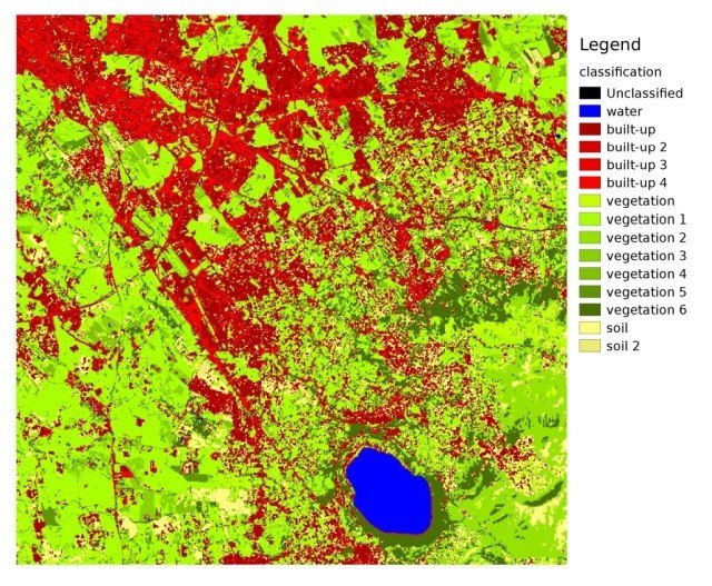
Landsat classification

I dati disponibili da U.S. Geological Survey

Una certa quantità di errori si può verificare nella classificazione della copertura del suolo (ad esempio alcuni pixel possono essere assegnati a una classe di copertura suolo sbagliata), a causa della somiglianza spettrale tra le classi, o per una definizione sbagliata della classe durante la raccolta ROI.

3.2.8. Valutazione dell’Accuratezza

Dopo il processo di classificazione, è utile valutare la precisione della classificazione copertura del suolo, al fine di identificare e misurare l’errore della mappa risultante. Solitamente, la valutazione dell’accuratezza è effettuata con il calcolo di una matrice di errore, che è una tabella che mette a confronto i dati di mappa con i dati di riferimento (ad esempio dati di verità a terra) per un certo numero di aree campione (Congalton e Green, 2009).

La seguente tabella è una matrice degli errori, dove k è il numero di classi identificate nella classificazione copertura del suolo, ed n è il numero totale di unità di campionamento raccolte. Le voci nella diagonale (aii) sono il numero di elementi correttamente classificati, mentre gli altri elementi sono errori di classificazione.

Scheme of Error Matrix

	Ground truth 1	Ground truth 2	…	Ground truth k	Total
Class 1	\(a_{11}\)	\(a_{12}\)	…	\(a_{1k}\)	\(a_{1+}\)
Class 2	\(a_{21}\)	\(a_{22}\)	…	\(a_{2k}\)	\(a_{2+}\)
…	…	…	…	…	…
Class k	\(a_{k1}\)	\(a_{k2}\)	…	\(a_{kk}\)	\(a_{k+}\)
Total	\(a_{+1}\)	\(a_{+2}\)	…	\(a_{+k}\)	\(n\)

Pertanto, è possibile calcolare la precisione complessiva come rapporto tra il numero di campioni correttamente classificate (la somma della diagonale maggiore), e il numero totale di unità di campionamento n (Congalton e Green, 2009).

Per ulteriori informazioni, sono disponibili liberamente i seguenti documenti: Landsat 7 Science Data User’s Handbook, Remote Sensing Note , or Wikipedia.

3.3. Image conversion to reflectance

This chapter provides information about the conversion to reflectance implemented in SCP.

3.3.1. Radianza al Sensore

**Radianza**è il “flusso di energia (principalmente irradiante o energia incidente) per angolo solido emesso da una superficie unitaria in una data direzione”, “Radiance è ciò che viene misurato sul sensore ed è in qualche modo dipendente dalla riflettanza” (NASA, 2011, p. 47).

Images such as Landsat or Sentinel-2 are composed of several bands and a metadata file which contains information required for the conversion to reflectance.

Landsat images are provided in radiance, scaled prior to output. for Landsat images Spectral Radiance at the sensor’s aperture (\(L_{\lambda}\), measured in [watts/(meter squared * ster * \(\mu m\))]) is given by (https://landsat.usgs.gov/Landsat8_Using_Product.php):

\[L_{\lambda} = M_{L} * Q_{cal} + A_{L}\]

where:

• \(M_{L}\) = fattore moltiplicativo Banda-specifico dai metadati Landsat (RADIANCE_MULT_BAND_x, dove x è il numero di banda)

• \(A_{L}\) = fattore additivo Banda-specifico dai metadati Landsat (RADIANCE_ADD_BAND_x, dove x è il numero della banda)

• \(Q_{cal}\) = Quantized and calibrated standard product pixel values (DN)

Sentinel-2 images (Level-1C) are already provided in Top Of Atmosphere (TOA) Reflectance, scaled prior to output (ESA, 2015).

3.3.2. Top Of Atmosphere (TOA) Reflectance

Images in radiance can be converted to Top Of Atmosphere (TOA) Reflectance (combined surface and atmospheric reflectance) in order to reduce the in between-scene variability through a normalization for solar irradiance. This TOA reflectance (\(\rho_{p}\)), which is the unitless ratio of reflected versus total power energy (NASA, 2011), is calculated by:

\[\rho_{p} = (\pi * L_{\lambda} * d^{2} )/ (ESUN_{\lambda} * cos\theta_{s})\]

where:

• \(L_{\lambda}\) = Radianza spettrale al sensore (at-satellite radiance)

• \(d\) = Earth-Sun distance in astronomical units (provided with Landsat 8 metadata file, and an excel file is available from http://landsathandbook.gsfc.nasa.gov/excel_docs/d.xls)

• \(ESUN_{\lambda}\) =Media della irradianza exo-atmosferica

• \(\theta_{s}\) = Angolo zenitale solare in gradi, che è uguale a \(\theta_{s}\) = 90° - \(\theta_{e}\) dove \(\theta_{e}\) is the Sun elevation

It is worth pointing out that Landsat 8 images are provided with band-specific rescaling factors that allow for the direct conversion from DN to TOA reflectance.

Sentinel-2 images are already provided in scaled TOA reflectance, which can be converted to TOA reflectance with a simple calculation using the Quantification Value provided in the metadata (see https://sentinel.esa.int/documents/247904/349490/S2_MSI_Product_Specification.pdf).

3.3.3. Surface Reflectance

The effects of the atmosphere (i.e. a disturbance on the reflectance that varies with the wavelength) should be considered in order to measure the reflectance at the ground.

Come descritto da Moran et al. (1992), the riflettanza della superfice terrestre (\(\rho\)) is:

\[\rho = [\pi * (L_{\lambda} - L_{p}) * d^{2}]/ [T_{v} * ( (ESUN_{\lambda} * cos\theta_{s} * T_{z} ) + E_{down} )]\]

where:

• \(L_{p}\) è la radinaza diffusa

• \(T_{v}\) è la trasmittanza atmosferica nella direzione di osservazione

• \(T_{z}\) è la trasmittanza atmosferica nella direzione di illuminazione

• \(E_{down}\) is the downwelling diffuse irradiance

Therefore, we need several atmospheric measurements in order to calculate \(\rho\) (physically-based corrections). Alternatively, it is possible to use image-based techniques for the calculation of these parameters, without in-situ measurements during image acquisition. It is worth mentioning that Landsat Surface Reflectance High Level Data Products for Landsat 8 are available (for more information read http://landsat.usgs.gov/CDR_LSR.php).

3.3.4. Correzione DOS1

The Dark Object Subtraction (DOS) è una famiglia di correzioni atmosferiche basati su immagini. Chavez (1996) spiega che “l’assunto di base è che nell’immagine alcuni pixel sono in completa ombra e loro radianza ricevuta satellite è dovuta a dispersione atmosferica (path radiance). Questa ipotesi è combinato con il fatto che pochissimi obiettivi sulla la superficie terrestre sono il nero assoluto, così l’ipotesi di uno percento come riflettanza minima è meglio di zero”. vale la pena di sottolineare che la precisione delle tecniche di image-based è in genere inferiore a correzioni basate fisicamente, ma sono molto utili quando misurazioni atmosferiche non sono disponibili e possono migliorare la stima di riflettanza della superficie terrestre The path radiance è data da (Sobrino, et al., 2004):

\[L_{p} = L_{min} - L_{DO1\%}\]

where:

• :

• \(L_{DO1\%}\) = radianza del Dark Object, assunto avere riflettanza 0.01

In particular for Landsat images:

\[L_{min} = M_{L} * DN_{min} + A_{L}\]

Sentinel-2 images are converted to radiance prior to DOS1 calculation.

La**radianza del Dark Object** è data da (Sobrino, et al., 2004):

\[L_{DO1\%} = 0.01 * [(ESUN_{\lambda} * cos\theta_{s} * T_{z} ) + E_{down}] * T_{v} / (\pi * d^{2})\]

Pertanto la radianza diffusa è:

\[L_{p} = M_{L} * DN_{min} + A_{L} - 0.01* [(ESUN_{\lambda} * cos\theta_{s} * T_{z} ) + E_{down}] * T_{v} / (\pi * d^{2})\]

Esistono varie tecniche DOS (e.g. DOS1, DOS2, DOS3, DOS4), basate su differenti assunzioni: math:T_{v}, \(T_{z}\) , and \(E_{down}\) . La tecnica più semplice è il DOS1, dove sono fatte le seguenti ipotesi (Moran et al., 1992):

• \(T_{v}\) = 1
• \(T_{z}\) = 1
• \(E_{down}\) = 0

Pertanto la radianza diffusa è:

\[L_{p} = M_{L} * DN_{min} + A_{L} - 0.01 * ESUN_{\lambda} * cos\theta_{s} / (\pi * d^{2})\]

E la risultante riflettanza superficiale terrestre è data da:

\[\rho = [\pi * (L_{\lambda} - L_{p}) * d^{2}]/ (ESUN_{\lambda} * cos\theta_{s})\]

ESUN [W /(m2 * \(\mu m\))] i valori per Landsat sono forniti dalla seguente tabella.

ESUN values for Landsat bands

Banda	Landsat 1 MSS*	Landsat 2 MSS*	Landsat 3 MSS*	Landsat 4 TM*	Landsat 5 TM*	Landsat 7 ETM+**
1				1983	1983	1970
2				1795	1796	1842
3				1539	1536	1547
4	1823	1829	1839	1028	1031	1044
5	1559	1539	1555	219.8	220	225.7
6	1276	1268	1291
7	880.1	886.6	887.9	83.49	83.44	82.06
8						1369

* from Chander, Markham, & Helder (2009)

** from http://landsathandbook.gsfc.nasa.gov/data_prod/prog_sect11_3.html

For Landsat 8, \(ESUN\) can be calculated as (from http://grass.osgeo.org/grass65/manuals/i.landsat.toar.html):

\[ESUN = (\pi * d^{2}) * RADIANCE\_MAXIMUM / REFLECTANCE\_MAXIMUM\]

dove RADIANCE_MAXIMUM e REFLECTANCE_MAXIMUM sono forniti.

ESUN [W /(m2 * \(\mu m\))] values for Sentinel-2 sensor (provided in image metadata) are illustrated in the following table.

ESUN values for Sentinel-2 bands

Banda	Sentinel-2
1	1913.57
2	1941.63
3	1822.61
4	1512.79
5	1425.56
6	1288.32
7	1163.19
8	1036.39
8A	955.19
9	813.04
10	367.15
11	245.59
12	85.25

ESUN [W /(m2 * \(\mu m\))] values for ASTER sensor are illustrated in the following table (from Finn, et al., 2012).

ESUN values for ASTER bands

Banda	ASTER
1	1848
2	1549
3	1114
4	225.4
5	86.63
6	81.85
7	74.85
8	66.49
9	59.85

Un esempio di confronto tra riflettanza TOA, riflettanza corretta con DOS1 e una Landsat Surface Reflectance High Level Data Products (ground truth) in Figure Firme spettrali di un pixel di costruito.

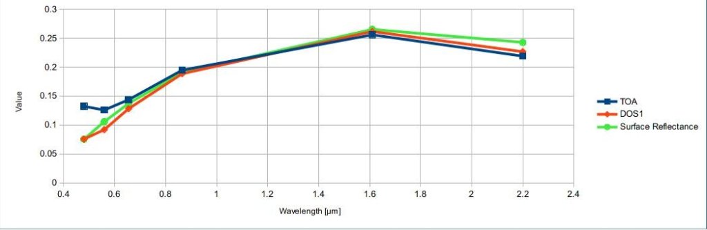
Firme spettrali di un pixel di costruito

confronto tra riflettanza TOA, riflettanza corretta con DOS1 e Landsat Surface Reflectance High Level Data Products

3.4. Conversion to Temperature

This chapter provides the basic information about the conversion to At-Satellite Brightness Temperature implemented in SCP and the estimation of Land Surface Temperature.

3.4.1. Conversione At-Satellite Brightness Temperature

For thermal bands, the conversion of DN to At-Satellite Brightness Temperature is given by (from https://landsat.usgs.gov/Landsat8_Using_Product.php):

\[T_{B} = K_{2} / ln[(K_{1} / L_{\lambda}) + 1]\]

where:

• \(K_{1}\) = Banda-specifica costante di conversione termica (in watts/meter squared * ster * \(\mu m\))

• \(K_{2}\) = Banda-specifica costante di conversione termica (in kelvin)

and \(L_{\lambda}\) is the Spectral Radiance at the sensor’s aperture, measured in watts/(meter squared * ster * \(\mu m\)).

The \(K_{1}\) and \(K_{2}\) constants for Landsat sensors are provided in the following table.

Thermal Conversion Constants for Landsat

Costante	Landsat 4*	Landsat 5*	Landsat 7**
\(K_{1}\)	671.62	607.76	666.09
\(K_{2}\)	1284.30	1260.56	1282.71

* from Chander & Markham (2003)

** from NASA (2011)

For Landsat 8, the \(K_{1}\) and \(K_{2}\) values are provided in the image metadata file.

\(K_{1}\) and \(K_{2}\) are calculated as (Jimenez-Munoz & Sobrino, 2010):

\[K_{1} = c_{1} / \lambda^{5}\]

\[K_{2} = c_{2} / \lambda\]

where (Mohr, Newell, & Taylor, 2015):

• \(c_{1}\) = first radiation constant = \(1.191 * 10^{-16} W m^{2} sr^{-1}\)
• \(c_{2}\) = second radiation constant = \(1.4388 * 10^{-2} m K\)

Therefore, for ASTER bands \(K_{1}\) and \(K_{2}\) are provided in the following table.

Thermal Conversion Constants for ASTER

Costante	Band 10	Band 11	Band 12	Band 13	Band 14
\(K_{1}\)	\(3.024 * 10^{3}\)	\(2.460 * 10^{3}\)	\(1.909 * 10^{3}\)	\(8.900 * 10^{2}\)	\(6.464 * 10^{2}\)
\(K_{2}\)	\(1.733 * 10^{3}\)	\(1.663 * 10^{3}\)	\(1.581 * 10^{3}\)	\(1.357 * 10^{3}\)	\(1.273 * 10^{3}\)

3.4.2. Estimation of Land Surface Temperature

Several studies have described the estimation of Land Surface Temperature. Land Surface Temperature can be calculated from At-Satellite Brightness Temperature \(T_{B}\) as (Weng, et al. 2004):

\[T = T_{B} / [ 1 + (\lambda * T_{B} / c_{2}) * ln(e) ]\]

where:

• \(\lambda\) = wavelength of emitted radiance
• \(c_{2} = h * c / s = 1.4388 * 10^{-2}\) m K
• \(h\) = Planck’s constant = \(6.626 * 10^{-34}\) J s
• \(s\) = Boltzmann constant = \(1.38 * 10^{-23}\) J/K
• \(c\) = velocity of light = \(2.998 * 10^{8}\) m/s

The values of \(\lambda\) for the thermal bands of Landsat and ASTER satellites can be calculated from the tables in Satellite Landsat and ASTER Satellite.

Several studies used NDVI for the estimation of land surface emissivity (Sobrino, et al., 2004); other studies used a land cover classification for the definition of the land surface emissivity of each class (Weng, et al. 2004). For instance, the emissivity (\(e\)) values of various land cover types are provided in the following table (from Mallick, et al. 2012).

Emissivity values

Land surface	Emissivity e
Soil	0.928
Erba	0.982
Asphalt	0.942
Concrete	0.937

3.5. References

• Chander, G. & Markham, B. 2003. Revised Landsat-5 TM radiometric calibration procedures and postcalibration dynamic ranges Geoscience and Remote Sensing, IEEE Transactions on, 41, 2674 - 2677
• Chavez, P. S. 1996. Image-Based Atmospheric Corrections - Revisited and Improved Photogrammetric Engineering and Remote Sensing, [Falls Church, Va.] American Society of Photogrammetry, 62, 1025-1036
• Congalton, R. and Green, K., 2009. Assessing the Accuracy of Remotely Sensed Data: Principles and Practices. Boca Raton, FL: CRC Press
• Didan, K.; Barreto Munoz, A.; Solano, R. & Huete, A. 2015. MODIS Vegetation Index User’s Guide. Collection 6, NASA

• ESA, 2015. Sentinel-2 User Handbook. Disponibile a https://sentinel.esa.int/documents/247904/685211/Sentinel-2_User_Handbook

• Finn, M.P., Reed, M.D, and Yamamoto, K.H. 2012. A Straight Forward Guide for Processing Radiance and Reflectance for EO-1 ALI, Landsat 5 TM, Landsat 7 ETM+, and ASTER. Unpublished Report from USGS/Center of Excellence for Geospatial Information Science, 8 p, http://cegis.usgs.gov/soil_moisture/pdf/A%20Straight%20Forward%20guide%20for%20Processing%20Radiance%20and%20Reflectance_V_24Jul12.pdf
• Fisher, P. F. and Unwin, D. J., eds. 2005. Representing GIS. Chichester, England: John Wiley & Sons
• JARS, 1993. Remote Sensing Note. Japan Association on Remote Sensing. Available at http://www.jars1974.net/pdf/rsnote_e.html
• Jimenez-Munoz, J. C. & Sobrino, J. A. 2010. A Single-Channel Algorithm for Land-Surface Temperature Retrieval From ASTER Data IEEE Geoscience and Remote Sensing Letters, 7, 176-179
• Johnson, B. A., Tateishi, R. and Hoan, N. T., 2012. Satellite Image Pansharpening Using a Hybrid Approach for Object-Based Image Analysis ISPRS International Journal of Geo-Information, 1, 228. Available at http://www.mdpi.com/2220-9964/1/3/228)
• Kruse, F. A., et al., 1993. The Spectral Image Processing System (SIPS) - Interactive Visualization and Analysis of Imaging spectrometer. Data Remote Sensing of Environment
• Mallick, J.; Singh, C. K.; Shashtri, S.; Rahman, A. & Mukherjee, S. 2012. Land surface emissivity retrieval based on moisture index from LANDSAT TM satellite data over heterogeneous surfaces of Delhi city International Journal of Applied Earth Observation and Geoinformation, 19, 348 - 358
• Mohr, P. J.; Newell, D. B. & Taylor, B. N. 2015. CODATA Recommended Values of the Fundamental Physical Constants: 2014 National Institute of Standards and Technology, Committee on Data for Science and Technology
• Moran, M.; Jackson, R.; Slater, P. & Teillet, P. 1992. Evaluation of simplified procedures for retrieval of land surface reflectance factors from satellite sensor output Remote Sensing of Environment, 41, 169-184
• NASA (Ed.) 2011. Landsat 7 Science Data Users Handbook Landsat Project Science Office at NASA’s Goddard Space Flight Center in Greenbelt, 186 http://landsathandbook.gsfc.nasa.gov/pdfs/Landsat7_Handbook.pdf
• NASA, 2013. Landsat 7 Science Data User’s Handbook. Available at http://landsathandbook.gsfc.nasa.gov
• Ready, P. and Wintz, P., 1973. Information Extraction, SNR Improvement, and Data Compression in Multispectral Imagery. IEEE Transactions on Communications, 21, 1123-1131
• Richards, J. A. and Jia, X., 2006. Remote Sensing Digital Image Analysis: An Introduction. Berlin, Germany: Springer.
• Sobrino, J.; Jiménez-Muñoz, J. C. & Paolini, L. 2004. Land surface temperature retrieval from LANDSAT TM 5 Remote Sensing of Environment, Elsevier, 90, 434-440
• USGS, 2015. Advanced Spaceborne Thermal Emission and Reflection Radiometer (ASTER) Level 1 Precision Terrain Corrected Registered At-Sensor Radiance Product (AST_L1T). AST_L1T Product User’s Guide. USGS EROS Data Center.
• Vermote, E. F.; Roger, J. C. & Ray, J. P. 2015. MODIS Surface Reflectance User’s Guide. Collection 6, NASA
• Weng, Q.; Lu, D. & Schubring, J. 2004. Estimation of land surface temperature–vegetation abundance relationship for urban heat island studies. Remote Sensing of Environment, Elsevier Science Inc., Box 882 New York NY 10159 USA, 89, 467-483