3. Breve Introdução ao Sensoriamento Remoto¶

3.1. Definições Básicas ¶

This chapter provides basic definitions about GIS and remote sensing. For other useful resources see Free and valuable resources about remote sensing and GIS.

Existem várias definições de SIG (Sistemas de Informação Geográfica), o qual não é simplesmente um programa. De um modo geral, os SIG são sistemas que permitem o uso da informação geográfica (dados com coordenadas espaciais). Particularmente, os SIG permitem a visualização, consulta, cálculo e análise dos dados espaciais, que são divididos principalmente em estrutura de dados vetorial ou raster. O vetor é formado por pontos, linhas ou polígonos, e cada objeto pode ter um ou mais valores de atributo; um raster é uma grade (ou imagem) onde cada célula/pixel tem um valor de atributo (Fisher e Unwin, 2005). Diversos programas SIG utilizam imagens raster oriundas do sensoriamento remoto.

3.1.2. Definição de Sensoriamento Remoto ¶

Uma definição geral para Sensoriamento Remoto é a que se refere a “ciência e tecnologia através da qual as características dos objectos de interesse podem ser identificadas, medidas ou analisadas sem haver o contato direto” (JARS, 1993).

Geralmente, o sensoriamento remoto trabalha com a medição da energia que é refletida a partir da superfície da Terra. Se a fonte da energia medida é o Sol, então é chamado de sensoriamento remoto passivo, e o resultado dessa medição pode ser uma imagem digital (Richards and Jia, 2006). Se a energia medida não é emitida pelo Sol, mas da plataforma orbital, então é definido como sensoriamento remoto ativo, tal como é o caso dos sensores radar, que funcionam na banda das microondas (Richards and Jia, 2006).

O espectro eletromagnético é “o sistema que classifica, de acordo com o comprimento de onda, toda a energia (desde os raios gama de comprimento de onda curto até às ondas de rádio de comprimento de onda longo) que se move, harmonicamente, à velocidade constante da luz” (NASA, 2013). Os sensores passivos medem a energia das regiões ópticas do espectro electromagnético: visível, infravermelho próximo (NIR), infravermelho médio e infravermelho termal (ver Figura Electromagnetic-Spectrum).

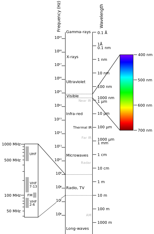
Electromagnetic-Spectrum

por Victor Blacus (versão SVG do ficheiro: Electromagnetic-Spectrum.png)

[CC-BY-SA-3.0 (http://creativecommons.org/licenses/by-sa/3.0)]

via Wikimedia Commons

http://commons.wikimedia.org/wiki/File%3AElectromagnetic-Spectrum.svg

A interação entre a energia solar e os materiais depende do comprimento de onda; a energia solar vai do Sol para a Terra e, depois, segue para o sensor. Ao longo desse caminho, a energia solar é (NASA, 2013):

Transmitida - A energia passa por uma mudança de sua velocidade, a qual é determinada pelo índice de refração para os dois meios em questão.
Absorvida - A energia é perdida para o objeto por meio de elétrons ou reações moleculares.
Refletida - A energia é reenviada inalterada para o espaço com o ângulo de incidência igual ao ângulo de reflexão. A reflectância de um corpo corresponde à razão entre a radiação refletida e a radiação incidente. O comprimento de onda refletido (não absorvido) determina a cor do objeto.
Dispersada - A direção de propagação da energia é modificada aleatoriamente. Dispersão de Rayleigh e de Mie são os dois principais tipos mais importantes de dispersão na atmosfera.
Emitida - Na realidade, a energia é inicialmente absorvida e depois reemitida, geralmente com um comprimento de onda mais longo. Assim, o objeto é aquecido por intermédio deste fenômeno.

3.1.3. Sensores ¶

Sensores podem estar à bordo de aviões ou satélites, medindo a radiação eletromagnética em intervalos específicos (geralmente chamados de bandas). Como resultado, as medidas são quantificadas e convertidas em uma imagem digital, onde cada elemento da imagem (i.e pixel) tem um valor discreto em unidades de Número Digital (ND) (NASA, 2013). As imagens resultantes possuem diferentes características (resoluções) dependendo do sensor. Há diversos tipos de resoluções:

Resolução espacial, normalmente medida em tamanho de pixel, “é o poder de resolução de um instrumento necessário para a discriminação de feições e é baseado no tamanho do detector, na distância focal e na altitude do sensor” (NASA, 2013); a resolução espacial também é denominada de resolução geométrica ou IFOV;
Resolução espectral, é o número e localização no espectro eletromagnético (definido por dois comprimentos de onda) das bandas espectrais (NASA, 2013) em sensores multiespectrais em que cada banda corresponde uma imagem;
Resolução radiométrica, geralmente medida em bits (dígitos binários), é o intervalo de valores de brilho disponível, de modo que na imagem corresponde ao alcance máximo de NDs; por exemplo, uma imagem com resolução de 8 bits apresenta 256 níveis de brilho (Richards and Jia, 2006);
Para sensores de satélites, há também a resolução temporal, que é o tempo necessário para o sensor revisitar a mesma área da superfície terrestre (NASA, 2013).

3.1.4. Radiância e Reflectância ¶

Sensores medem a radiância, que corresponde ao brilho numa determinada direção em relação ao sensor; é útil para definir também a reflectância como a razão da energia refletida versus o poder total da energia.

3.1.5. Assinatura Espectral ¶

A assinatura espectral é a reflectância em função do comprimento de onda (ver Figura Curvas de Reflectância Espectral de Quatro Alvos Diferentes); cada material tem uma assinatura única, podendo ser usado em uma classificação (NASA, 2013).

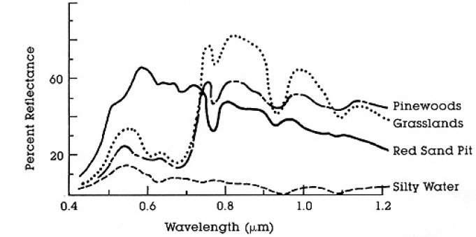
Curvas de Reflectância Espectral de Quatro Alvos Diferentes

(da NASA, 2013)`

3.1.6. Satélite Landsat ¶

Landsat é um conjunto de satélite multiespectrais desenvolvidos pela NASA (sigla em inglês de Administração Nacional da Aeronáutica e Espaço dos EUA), desde o início dos anos 1970.

Imagens Landsat são muito utilizadas em pesquisas ambientais. As resoluções dos sensores Landsat 4 e Landsat 5 são relatados na tabela a seguir (de http://landsat.usgs.gov/band_designations_landsat_satellites.php); além disso, a resolução temporal é de 16 dias (NASA, 2013).

Landsat 4 and Landsat 5 Bands

Bandas Landsat 4, Landsat 5	Comprimento de onda [micrômetros]	Resolução [metros]
Banda 1 - Azul	0.45 - 0.52	30
Banda 2 - Verde	0.52 - 0.60	30
Banda 3 - Vermelho	0.63 - 0.69	30
Banda 4 - Infravermelho Próximo (NIR)	0.76 - 0.90	30
Banda 5 - SWIR	1.55 - 1.75	30
Banda 6 - Infravermelho Termal	10.40 - 12.50	120 (reamostrada para 30)
Banda 7 - SWIR	2.08 - 2.35	30

As resoluções do sensor Landsat 7 estão relatadas na tabela a seguir (de http://landsat.usgs.gov/band_designations_landsat_satellites.php); além disso, a resolução temporal Landsat é de 16 dias (NASA, 2013).

Landsat 7 Bands

Bandas Landsat 7	Comprimento de onda [micrômetros]	Resolução [metros]
Banda 1 - Azul	0.45 - 0.52	30
Banda 2 - Verde	0.52 - 0.60	30
Banda 3 - Vermelho	0.63 - 0.69	30
Banda 4 - Infravermelho Próximo (NIR)	0.77 - 0.90	30
Banda 5 - SWIR	1.57 - 1.75	30
Banda 6 - Infravermelho Termal	10.40 - 12.50	60 (reamostrada para 30)
Banda 7 - SWIR	2.09 - 2.35	30
Banda 8 - Pancromática	0.52 - 0.90	15

As resoluções do sensor Landsat 8 estão relatadas na tabela a seguir (de http://landsat.usgs.gov/band_designations_landsat_satellites.php); além disso, a resolução temporal Landsat é de 16 dias (NASA, 2013).

Landsat 8 Bands

Bandas Landsat 8	Comprimento de onda [micrômetros]	Resolução [metros]
Banda 1 - Zona costeira e aerossóis	0.43 - 0.45	30
Banda 2 - Azul	0.45 - 0.51	30
Banda 3 - Verde	0.53 - 0.59	30
Banda 4 - Vermelho	0.64 - 0.67	30
Banda 5 - Infravermelho Próximo (NIR)	0.85 - 0.88	30
Banda 6 - SWIR 1	1.57 - 1.65	30
Banda 7 - SWIR 2	2.11 - 2.29	30
Banda 8 - Pancromática	0.50 - 0.68	15
Banda 9 - Cirrus (deteccção de nuvens)	1.36 - 1.38	30
Banda 10 - Infravermelho Termal (TIRS) 1	10.60 - 11.19	100 (reamostrada para 30)
Banda 11 - Infravermelho Termal (TIRS) 2	11.50 - 12.51	100 (reamostrada para 30)

A vast archive of images is freely available from the U.S. Geological Survey . For more information about how to freely download Landsat images read this .

Images are identified with the paths and rows of the WRS (Worldwide Reference System for Landsat ).

3.1.7. Satélite Sentinel-2 ¶

Sentinel-2 é um satélite multiespectral desenvolvido pela Agência Espacial Europeia (ESA) no formato de serviços de monitoramento da terra Copernicus. Sentinel-2 têm 13 bandas espectrais com resolução espacial de 10m, 20m e 60m de acordo com a banda, como ilustrado na tabela a seguir (ESA, 2015).

Sentinel-2 Bands

Bandas do Sentinel-2	Comprimento de Onda Central [micrômetros]	Resolução [metros]
Banda 1 - Zona costeira e aerossóis	0.443	60
Banda 2 - Azul	0.490	10
Banda 3 - Verde	0.560	10
Banda 4 - Vermelho	0.665	10
Banda 5 - Red Edge (Vegetação)	0.705	20
Banda 6 - Red Edge (Vegetação)	0.740	20
Banda 7 - Red Edge (Vegetação)	0.783	20
Banda 8 - NIR	0.842	10
Banda 8A - Red Edge (Vegetação)	0.865	20
Banda 9 - Vapor d’água	0.945	60
Banda 10 - SWIR - Cirrus	1.375	60
Banda 11 - SWIR	1.610	20
Banda 12 - SWIR	2.190	20

As imagens Sentinel-2 estão disponibilizadas gratuitamente no site da ESA https://scihub.esa.int/dhus/

3.1.8. ASTER Satellite ¶

The ASTER (Advanced Spaceborne Thermal Emission and Reflection Radiometer) satellite was launched in 1999 by a collaboration between the Japanese Ministry of International Trade and Industry (MITI) and the NASA. ASTER has 14 bands whose spatial resolution varies with wavelength: 15m in the visible and near-infrared, 30m in the short wave infrared, and 90m in the thermal infrared (USGS, 2015). ASTER bands are illustrated in the following table (due to a sensor failure SWIR data acquired since April 1, 2008 is not available ). An additional band 3B (backwardlooking near-infrared) provides stereo coverage.

ASTER Bands

ASTER Bands	Comprimento de onda [micrômetros]	Resolução [metros]
Band 1 - Green	0.52 - 0.60	15
Band 2 - Red	0.63 - 0.69	15
Band 3N - Near Infrared (NIR)	0.78 - 0.86	15
Band 4 - SWIR 1	1.60 - 1.70	30
Band 5 - SWIR 2	2.145 - 2.185	30
Band 6 - SWIR 3	2.185 - 2.225	30
Band 7 - SWIR 4	2.235 - 2.285	30
Band 8 - SWIR 5	2.295 - 2.365	30
Band 9 - SWIR 6	2.360 - 2.430	30
Band 10 - TIR 1	8.125 - 8.475	90
Band 11 - TIR 2	8.475 - 8.825	90
Band 12 - TIR 3	8.925 - 9.275	90
Band 13 - TIR 4	10.25 - 10.95	90
Band 14 - TIR 5	10.95 - 11.65	90

3.1.9. MODIS Products ¶

The MODIS (Moderate Resolution Imaging Spectroradiometer) is an instrument operating on the Terra and Aqua satellites launched by NASA in 1999 and 2002 respectively. Its temporal resolutions allows for viewing the entire Earth surface every one to two days, with a swath width of 2,330. Its sensors measure 36 spectral bands at three spatial resolutions: 250m, 500m, and 1,000m (see https://lpdaac.usgs.gov/dataset_discovery/modis).

Several products are available, such as surface reflectance and vegetation indices. In this manual we are considering the surface reflectance bands available at 250m and 500m spatial resolution (Vermote, Roger, & Ray, 2015).

MODIS Bands

MODIS Bands	Comprimento de onda [micrômetros]	Resolução [metros]
Band 1 - Red	0.62 - 0.67	250 - 500
Band 2 - Near Infrared (NIR)	0.841 - 0.876	250 - 500
Band 3 - Blue	0.459 - 0.479	500
Band 4 - Green	0.545 - 0.565	500
Band 5 - SWIR 1	1.230 - 1.250	500
Band 6 - SWIR 2	1.628 - 1.652	500
Band 7 - SWIR 3	2.105 - 2.155	500

The following products (Version 6, see https://lpdaac.usgs.gov/dataset_discovery/modis/modis_products_table) are available for download (Vermote, Roger, & Ray, 2015):

MOD09GQ: daily reflectance at 250m spatial resolution from Terra MODIS;
MYD09GQ: daily reflectance at 250m spatial resolution from Aqua MODIS;
MOD09GA: daily reflectance at 500m spatial resolution from Terra MODIS;
MYD09GA: daily reflectance at 500m spatial resolution from Aqua MODIS;
MOD09Q1: reflectance at 250m spatial resolution, which is a composite of MOD09GQ (each pixel contains the best possible observation during an 8-day period);
MYD09Q1: reflectance at 250m spatial resolution, which is a composite of MYD09GQ (each pixel contains the best possible observation during an 8-day period);
MOD09A1: reflectance at 250m spatial resolution, which is a composite of MOD09GA (each pixel contains the best possible observation during an 8-day period);
MYD09A1: reflectance at 250m spatial resolution, which is a composite of MYD09GA (each pixel contains the best possible observation during an 8-day period);

3.1.10. Composição colorida ¶

Muitas vezes, uma combinação é criada a partir de três imagens monocromáticas individuais, em que para cada um é atribuída determinada cor; isso é definido como composição colorida e é útil na fotointerpretaçao (NASA, 2013). Composições coloridas são geralmente expressas como:

“R G B = Br Bg Bb”

onde:

R significa Vermelho;
G significa Verde;
B significa Azul;
Br é o número de banda associado à cor Vermelho;
Bg é o número de banda associado à cor Verde;
Bb é o número de banda associado à cor Azul.

The following Figure Composição colorida da imagem Landsat 8 shows a color composite “R G B = 4 3 2” of a Landsat 8 image (for Landsat 7 the same color composite is R G B = 3 2 1; for Sentinel-2 is R G B = 4 3 2) and a color composite “R G B = 5 4 3” (for Landsat 7 the same color composite is R G B = 4 3 2; for Sentinel-2 is R G B = 8 4 3). The composite “R G B = 5 4 3” is useful for the interpretation of the image because vegetation pixels appear red (healthy vegetation reflects a large part of the incident light in the near-infrared wavelength, resulting in higher reflectance values for band 5, thus higher values for the associated color red).

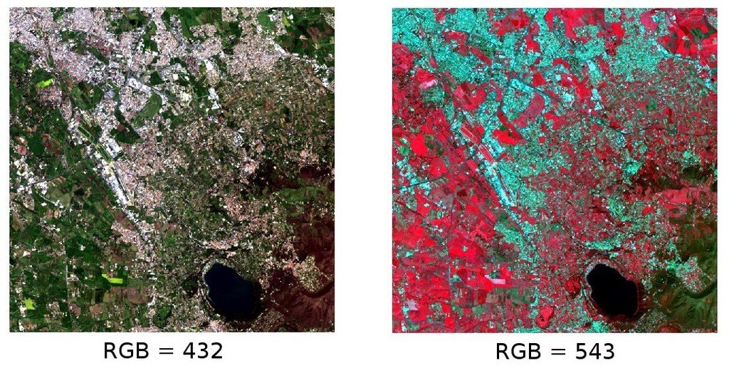
Composição colorida da imagem Landsat 8

Dados disponibilizados pelo Serviço Geológico dos EUA

3.1.11. Principal Component Analysis ¶

Principal Component Analysis (PCA) is a method for reducing the dimensions of measured variables (bands) to the principal components (JARS, 1993).

Th principal component transformation provides a new set of bands (principal components) having the following characteristic: principal components are uncorrelated; each component has variance less than the previous component. Therefore, this is an efficient method for extracting information and data compression (Ready and Wintz, 1973).

Given an image with N spectral bands, the principal components are obtained by matrix calculation (Ready and Wintz, 1973; Richards and Jia, 2006):

\[Y = D^t X\]

onde:

\(Y\) = vector of principal components
\(D\) = matrix of eigenvectors of the covariance matrix \(C_x\) in X space
\(t\) denotes vector transpose

And \(X\) is calculated as:

\[X = P - M\]

\(P\) = vector of spectral values associated with each pixel
\(M\) = vector of the mean associated with each band

Thus, the mean of \(X\) associated with each band is 0. \(D\) is formed by the eigenvectors (of the covariance matrix \(C_x\)) ordered as the eigenvalues from maximum to minimum, in order to have the maximum variance in the first component. This way, the principal components are uncorrelated and each component has variance less than the previous component(Ready and Wintz, 1973).

Usually the first two components contain more than the 90% of the variance. For example, the first principal components can be displayed in a Composição colorida for highlighting Cobertura da Terra classes, or used as input for Classificação Supervisionada.

3.1.12. Pan-sharpening ¶

Pan-sharpening is the combination of the spectral information of multispectral bands (MS), which have lower spatial resolution (for Landsat bands, spatial resolution is 30m), with the spatial resolution of a panchromatic band (PAN), which for Landsat 7 and 8 it is 15m. The result is a multispectral image with the spatial resolution of the panchromatic band (e.g. 15m). In SCP, a Brovey Transform is applied, where the pan-sharpened values of each multispectral band are calculated as (Johnson, Tateishi and Hoan, 2012):

\[MSpan = MS * PAN / I\]

onde \(I\) é intensidade, que é uma função de bandas multiespectrais.

The following weights for I are defined, basing on several tests performed using the SCP. For Landsat 8, Intensity is calculated as:

\[I = (0.42 * Blue + 0.98 * Green + 0.6 * Red ) / 2\]

Para Landsat 7, Intensidade é calculada como:

\[I = (0.42 * Blue + 0.98 * Green + 0.6 * Red + NIR) / 3\]

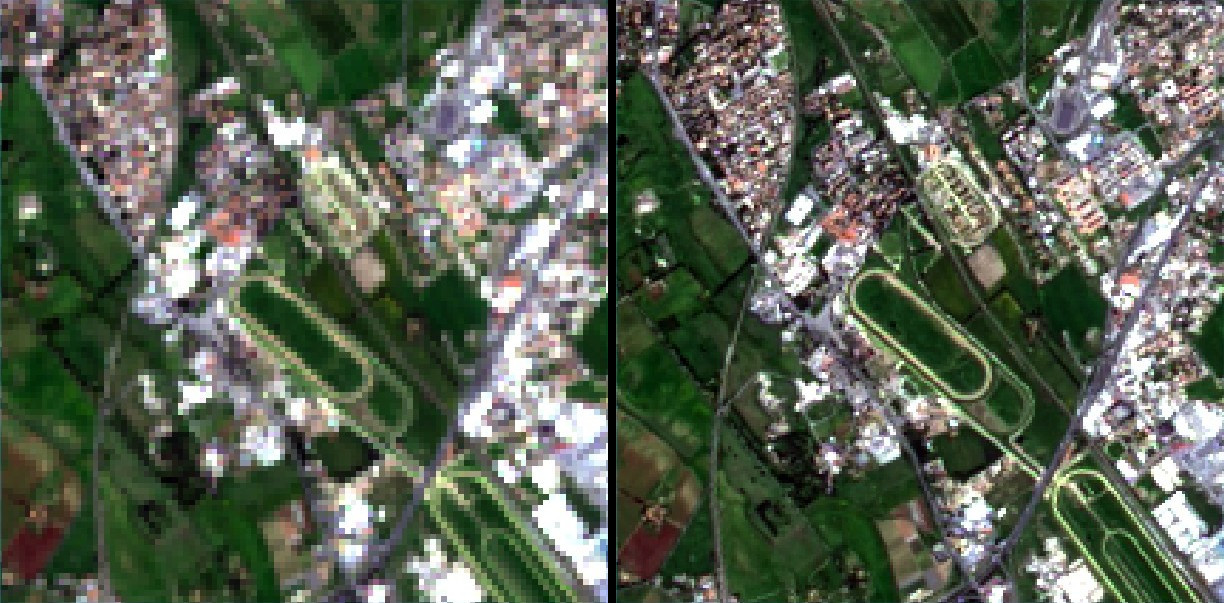
Exemplo de pan-sharpening de uma imagem Landsat 8. À esquerda, bandas multiespectrais originais (30m); à direita, bandas pan-sharpened (15m)

Dados disponibilizados pelo Serviço Geológico dos EUA

3.1.13. Spectral Indices ¶

Spectral indices are operations between spectral bands that are useful for extracting information such as vegetation cover (JARS, 1993). One of the most popular spectral indices is the Normalized Difference Vegetation Index (NDVI), defined as (JARS, 1993):

\[NDVI = ( NIR - Red ) / ( NIR + Red )\]

NDVI values range from -1 to 1. Dense and healthy vegetation show higher values, while non-vegetated areas show low NDVI values.

Another index is the Enhanced Vegetation Index (EVI) which attempts to account for atmospheric effects such as path radiance calculating the difference between the blue and the red bands (Didan,et al., 2015). EVI is defined as:

\[EVI = G ( NIR - Red ) / ( NIR + C_1 Red - C_2 Blue + L)\]

where: \(G\) is a scaling factor, \(C_1\) and \(C_2\) are coefficients for the atmospheric effects, and \(L\) is a factor for accounting the differential NIR and Red radiant transfer through the canopy. Typical coefficient values are: \(G = 2.5\), \(L = 1\), \(C_1 = 6\), \(C_2 = 7.5\) (Didan,et al., 2015).

3.2. Definições de Classificação Supervisionada ¶

Este capítulo fornece definições básicas sobre classificações supervisionadas.

3.2.1. Cobertura da Terra ¶

Cobertura da terra é o material no chão, tal como solo, vegetação, água, asfalto, etc. (Fisher e Unwin, 2005). Dependendo das resoluções do sensor, o número e tipo de classes de cobertura da terra identificadas na imagem podem variar significativamente.

3.2.2. Classificação Supervisionada ¶

Uma classificação semi-automática (e também classificação supervisionada) é uma técnica de processamento de imagem que permite a identificação de materiais em uma imagem, de acordo com as suas assinaturas espectrais. Há vários tipos de algoritmos de classificação, mas a proposta geral é produzir um mapa temático de cobertura da terra.

Processamento de imagem e análise espacial em SIG exigem programa específico tal como o Semi-Automatic Classification Plugin para QGIS.

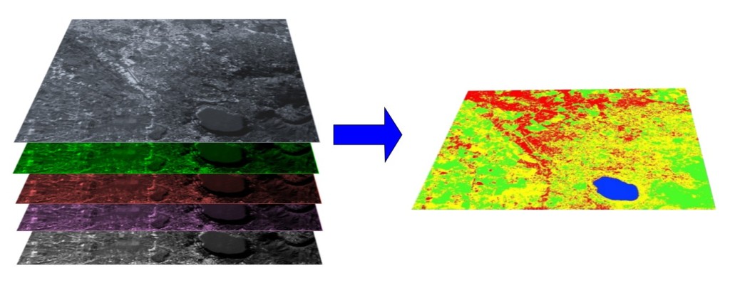
_images/multispectral_classification.jpg

A multispectral image processed to produce a land cover classification

(Landsat image provided by USGS)

3.2.3. Áreas de Treinamento ¶

Geralmente, classificações supervisionadas exigem que o usuário selecione uma ou mais Regiões de Interesse (ROIs, também chamadas de Áreas de Treinamento) para cada classe de cobertura da terra identificada na imagem. ROIs são polígonos desenhados sobre áreas homogêneas da imagem que sobrepõe pixels pertentecentes à mesma classe de cobertura da terra.

3.2.3.1. Region Growing Algorithm¶

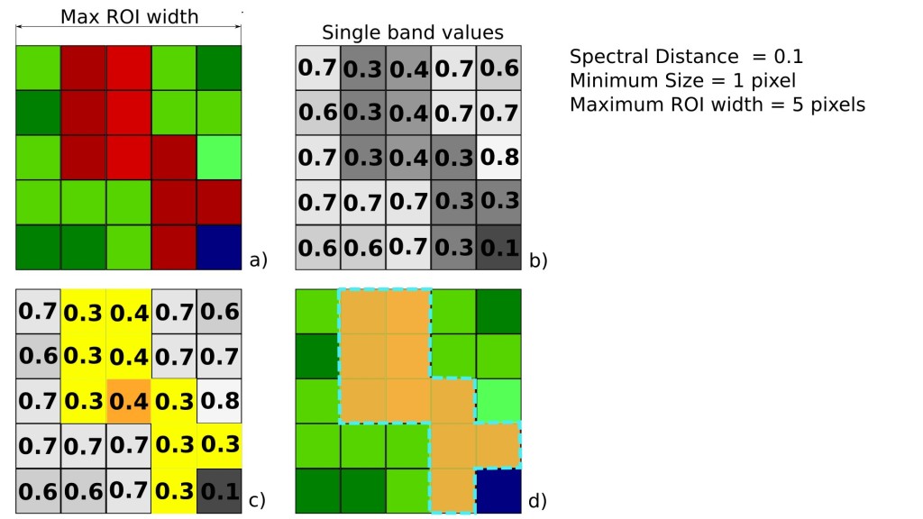
The Region Growing Algorithm allows to select pixels similar to a seed one, considering the spectral similarity (i.e. spectral distance) of adjacent pixels. In SCP the Region Growing Algorithm is available for the training area creation. The parameter distance is related to the similarity of pixel values (the lower the value, the more similar are selected pixels) to the seed one (i.e. selected clicking on a pixel). An additional parameter is the maximum width, which is the side length of a square, centred at the seed pixel, which inscribes the training area (if all the pixels had the same value, the training area would be this square). The minimum size is used a constraint (for every single band), selecting at least the pixels that are more similar to the seed one until the number of selected pixels equals the minimum size.

In figure Region growing example the central pixel is used as seed (image a) for the region growing of one band (image b) with the parameter spectral distance = 0.1; similar pixels are selected to create the training area (image c and image d).

Region growing example

3.2.4. Classes e Macroclasses ¶

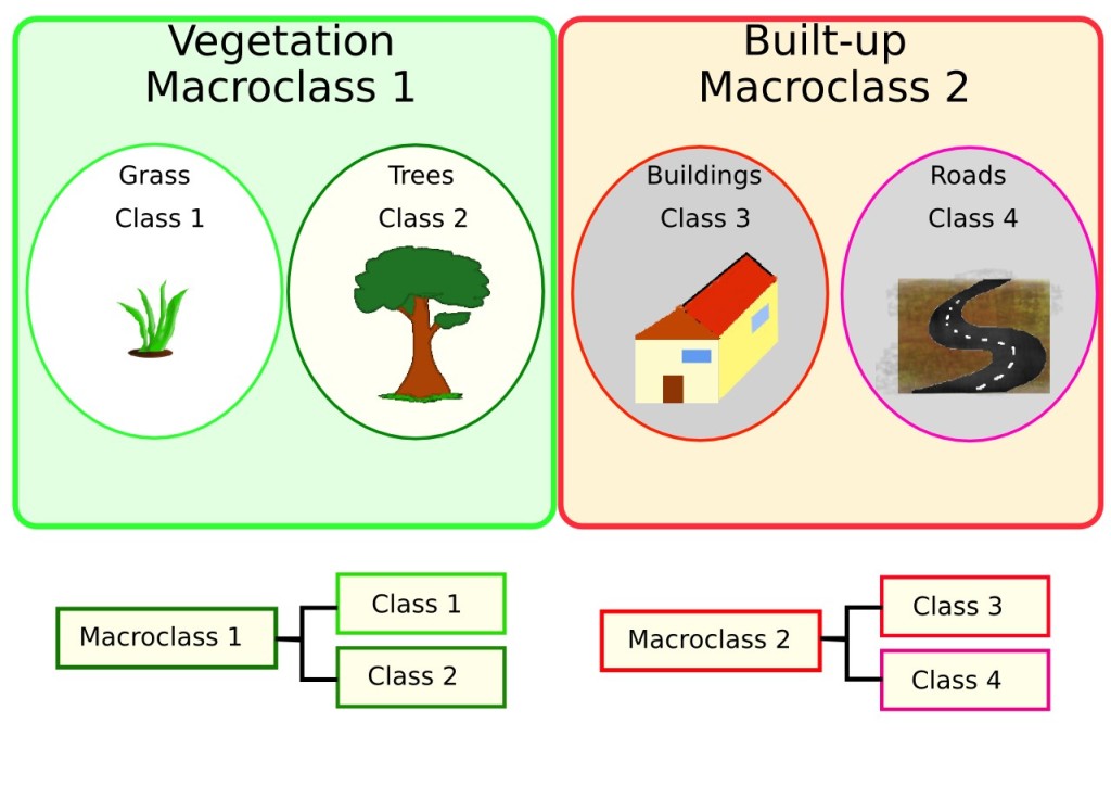
Land cover classes are identified with an arbitrary ID code (i.e. Identifier). SCP allows for the definition of Macroclass ID (i.e. MC ID) and Class ID (i.e. C ID), which are the identification codes of land cover classes. A Macroclass is a group of ROIs having different Class ID, which is useful when one needs to classify materials that have different spectral signatures in the same land cover class. For instance, one can identify grass (e.g. ID class = 1 and Macroclass ID = 1 ) and trees (e.g. ID class = 2 and Macroclass ID = 1 ) as vegetation class (e.g. Macroclass ID = 1 ). Multiple Class IDs can be assigned to the same Macroclass ID, but the same Class ID cannot be assigned to multiple Macroclass IDs, as shown in the following table.

Example of Macroclasses

Nome da Macroclasse	ID da Macroclasse	Nome da Classe	ID da Classe
Vegetação	1	Gramado	1
Vegetação	1	Árvores	2
Construído	2	Buildings	3
Construído	2	Roads	4

Portanto, as Classes são subconjuntos de uma Macroclasse, conforme ilustrado na Figura Examplo de uma Macroclasse.

Examplo de uma Macroclasse

Se o uso da Macroclasse não é exigido para o propósito do estudo, então, a mesma Macroclasse ID pode ser definida para todos os ROIs (e.g. Macroclasse ID = 1 ) e os valores de Macroclasse são ignorados no processo de classificação.

3.2.5. Algoritmos de Classificação ¶

The spectral signatures (spectral characteristics) of reference land cover classes are calculated considering the values of pixels under each ROI having the same Class ID (or Macroclass ID). Therefore, the classification algorithm classifies the whole image by comparing the spectral characteristics of each pixel to the spectral characteristics of reference land cover classes. SCP implements the following classification algorithms.

3.2.5.1. Mínima Distância¶

O algoritmo Mínima Distância calcula a distância Euclidiana \(d(x, y)\) entre assinaturas espectrais de pixels da imagem e assinaturas espectrais de treinamento, de acordo com a seguinte equação:

\[d(x, y) = \sqrt{ \sum_{i=1}^{n} (x_i - y_i)^2}\]

onde:

\(x\) = assinatura espectral vetorial de um pixel na imagem;
\(y\) = assinatura espectral vetorial de uma área de treinamento;
\(n\) = numero de bandas da imagem.

Assim, a distância é calculada para cada pixel na imagem, associando-o à classe que apresentar a assinatura espectral mais próxima, de acordo com a função discriminante (adaptado de Richards e Jia, 2006):

\[x \in C_k \iff d(x, y_k) < d(x, y_j) \forall k \neq j\]

onde:

\(C_k\) = classe de cobertura da terra \(k\);
\(y_k\) = assinatura espectral da classe \(k\);
\(y_j\) = assinatura espectral da classe \(j\).

É possível definir um limiar \(T_i\) em ordem para excluir os pixels abaixo desse valor da classificação:

\[ \begin{align}\begin{aligned}x \in C_k \iff d(x, y_k) < d(x, y_j) \forall k \neq j\\and\\d(x, y_k) < T_i\end{aligned}\end{align} \]

3.2.5.2. Máxima Verossimilhança¶

O algoritmo Máxima Verossimilhança calcula as distribuições de probabilidade para as classes, relacionados com o teorema de Baye’s, estimando se um pixel pertence a uma classe de cobertura da terra. Em particular, as distribuições de probabilidade para as classes assumem a forma de modelos normais multivariados ( Richards & Jia , 2006 ). Com a finalidade de utilizar este algoritmo, um número suficiente de pixels é exigido para cada área de treinamento permitindo o cálculo da matriz de covariância. A função discriminante, descrita por Richards e Jia (2006 ), é calculada para cada pixel como:

\[g_k(x) = \ln p(C_k) - \frac{1}{2} \ln | \Sigma_{k} | - \frac{1}{2} (x - y_k)^t \Sigma_{k}^{-1} (x - y_k)\]

onde:

\(C_k\) = classe de cobertura da terra \(k\);
\(x\) = assinatura espectral vetorial ou pixel de uma imagem;
\(p(C_k)\) = probabilidade da classe correta ser \(C_k\);
\(| \Sigma_{k} |\) = determinante da matriz de covariância dos dados na classe \(C_k\);
\(\Sigma_{k}^{-1}\) = inverso da matriz de covariância;
\(y_k\) = assinatura espectral vetorial da classe \(k\).

Portanto:

\[x \in C_k \iff g_k(x) > g_j(x) \forall k \neq j\]

Maximum Likelihood example

Além disso, é possível definir um limite para a função discriminante para excluir pixels abaixo deste valor da classificação. Considerando-se um limiar \(T_i\) a condição da classificação torna-se :

\[ \begin{align}\begin{aligned}x \in C_k \iff g_k(x) > g_j(x) \forall k \neq j\\and\\g_k(x) > T_i\end{aligned}\end{align} \]

A máxima verossimilhança é uma das classificações supervisionadas mais comuns, no entanto, o processo de classificação pode ser mais lento do que Mínima Distância.

3.2.5.3. Spectral Angle Mapping¶

O Mapeamento por Ângulo Espectral calcula o ângulo espectral entre assinaturas espectrais de pixels da imagem e assinaturas espectrais de treinamento. O ângulo espectral \(\theta\) é definido como (Kruse et al., 1993):

\[\theta(x, y) = \cos^{-1} \left( \frac{ \sum_{i=1}^{n} x_i y_i } { \left( \sum_{i=1}^{n} x_i^2 \right)^\frac{1}{2} * \left( \sum_{i=1}^{n} y_i^2 \right)^\frac{1}{2} } \right)\]

Where

\(x\) = assinatura espectral vetorial de um pixel na imagem;
\(y\) = assinatura espectral vetorial de uma área de treinamento;
\(n\) = numero de bandas da imagem.

Por conseguinte, um pixel pertence à classe que tem o menor ângulo, que é:

\[x \in C_k \iff \theta(x, y_k) < \theta(x, y_j) \forall k \neq j\]

onde:

\(C_k\) = classe de cobertura da terra \(k\);
\(y_k\) = assinatura espectral da classe \(k\);
\(y_j\) = assinatura espectral da classe \(j\).

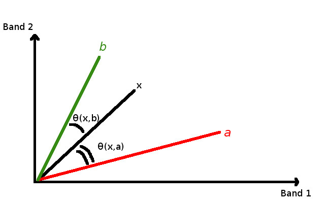
Spectral Angle Mapping example

A fim de excluir os pixels abaixo deste valor a partir da classificação é possível definir um limiar \(T_i\):

\[ \begin{align}\begin{aligned}x \in C_k \iff \theta(x, y_k) < \theta(x, y_j) \forall k \neq j\\and\\\theta(x, y_k) < T_i\end{aligned}\end{align} \]

O Mapeamento por Ângulo Espectral é largamento utilizado, especialmente com dados hiperespectrais.

3.2.5.4. Parallelepiped Classification¶

Parallelepiped classification is an algorithm that considers a range of values for each band, forming a multidimensional parallelepiped that defines a land cover class. A pixel is classified if the values thereof are inside a parallelepiped. One of the major drawbacks is that pixels whose signatures lie in the overlapping area of two or more parallelepipeds cannot be classified (Richards and Jia, 2006).

3.2.5.5. Land Cover Signature Classification¶

Land Cover Signature Classification is available in SCP (see Land Cover Signature Classification). This classification allows for the definition of spectral thresholds for each training input signature (a minimum value and a maximum value for each band). The thresholds of each training input signature define a spectral region belonging to a certain land cover class.

Spectral signatures of image pixels are compared to the training spectral signatures; a pixel belongs to class X if pixel spectral signature is completely contained in the spectral region defined by class X. In case of pixels falling inside overlapping regions or outside any spectral region, it is possible to use additional classification algorithms (i.e. Mínima Distância, Máxima Verossimilhança, Spectral Angle Mapping) considering the spectral characteristics of the original input signature.

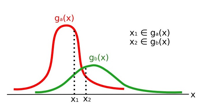
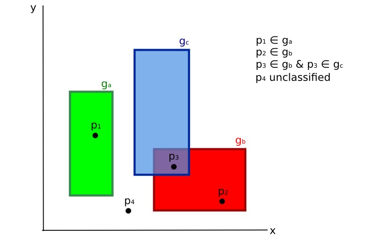
In the following image, a scheme illustrates the Land Cover Signature Classification for a simple case of two spectral bands \(x\) and \(y\). User defined spectral regions define three classes (\(g_a\), \(g_b\), and \(g_c\)). Point \(p_1\) belongs to class \(g_a\) and point \(p_2\) belongs to class \(g_b\). However, point \(p_3\) is inside the spectral regions of both classes \(g_b\) and \(g_c\) (overlapping regions); in this case, point \(p_3\) will be unclassified or classified according to an additional classification algorithm. Point \(p_4\) is outside any spectral region, therefore it will be unclassified or classified according to an additional classification algorithm. Given that point \(p_4\) belongs to class \(g_c\), the spectral region thereof could be extended to include point \(p_4\) .

Land cover signature classification

This is similar to Parallelepiped Classification, with the exception that spectral regions are defined by user, and can be assigned independently for the upper and lower bounds. One can imagine spectral regions as the set of all the spectral signatures of pixels belonging to one class.

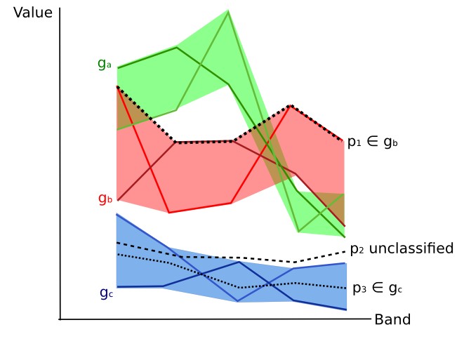
In figure Plot of spectral ranges the spectral ranges of three classes (\(g_a\), \(g_b\), and \(g_c\)) are displayed; the colored lines inside the ranges (i.e. semi-transparent area) represent the spectral signatures of pixels that defined the upper and lower bounds of the respective ranges. Pixel \(p_1\) (dotted line) belongs to class \(g_b\) because the spectral signature thereof is completely inside the range of class \(g_b\) (in the upper limit); pixel \(p_2\) (dashed line) is unclassified because the spectral signature does not fall completely inside any range; pixel \(p_3\) (dotted line) belongs to class \(g_a\).

_images/land_cover_signature_classification_plot.jpg

Plot of spectral ranges

It is worth noticing that these spectral thresholds can be applied to any spectral signature, regardless of spectral characteristics thereof; this function can be very useful for separating similar spectral signatures that differ only in one band, defining thresholds that include or exclude specific signatures. In fact, classes are correctly separated if the spectral ranges thereof are not overlapping at least in one band. Of course, even if spectral regions are overlapping, chances are that no pixel will fall inside the overlapping region and be misclassified; which is the upper (or lower) bound of a range do not imply the existence, in the image, of any spectral signature having the maximum (or minimum) range values for all the bands (for instance pixel \(p_1\) of figure Plot of spectral ranges could not exist).

One of the main benefit of the Land Cover Signature Classification is that it is possible to select pixels and and include the signature thereof in a spectral range; therefore, the classification should be the direct representation of the class expected for every spectral signature. This is very suitable for the classification of a single land cover class (defined by specific spectral thresholds), and leave unclassified the rest of the image that is of no interest for the purpose of the classification.

3.2.5.6. Algorithm raster¶

An algorithm raster represents the “distance” (according to the definition of the classification algorithm) of an image pixel to a specific spectral signature.

In general, an algorithm raster is produced for every spectral signature used as training input. The value of every pixel is the result of the algorithm calculation for a specific spectral signature. Therefore, a pixel belongs to class X if the value of the algorithm raster corresponding to class X is the lowest in case of Mínima Distância or Spectral Angle Mapping (or highest in case of Máxima Verossimilhança).

Given a classification, a combination of algorithm rasters can be produced, in order to create a raster with the lowest “distances” (i.e. pixels have the value of the algorithm raster corresponding to the class they belong in the classification). Therefore, this raster can be useful to identify pixels that require the collection of more similar spectral signatures (see Classification preview).

3.2.6. Distância Espectral ¶

It is useful to evaluate the spectral distance (or separability) between training signatures or pixels, in order to assess if different classes that are too similar could cause classification errors. The SCP implements the following algorithms for assessing similarity of spectral signatures.

3.2.6.1. Distância Jeffries-Matusita¶

A Distância Jeffries-Matusita calcula a separabilidade de um par de distribuições de probabilidade. Isto pode ser particularmente significativo para estimar os resultados de classificações Máxima Verossimilhança.

A Distância Jeffries-Matusita \(J_{xy}\) é calculada como (Richards e Jia, 2006):

\[J_{xy} = 2 \left( 1 - e^{-B} \right)\]

onde:

\[B = \frac{1}{8} (x - y)^t \left( \frac{\Sigma_{x} + \Sigma_{y}}{2} \right)^{-1} (x - y) + \frac{1}{2} \ln \left( \frac{ | \frac{ \Sigma_{x} + \Sigma_{y}}{2} | }{ | \Sigma_{x} |^{\frac{1}{2}} | \Sigma_{y} |^{\frac{1}{2}} } \right)\]

onde:

\(x\) = primeira assinatura espectral vetorial;
\(y\) = segunda assinatura espectral vetorial;
\(\Sigma_{x}\) = amostra da matriz de covariância \(x\);
\(\Sigma_{y}\) = amostra da matriz de covariância \(y\);

A Distância Jeffries-Matusita é assintótica a 2 quando as assinaturas são completamente diferentes, e tende a 0 quando as assinaturas são idênticas.

3.2.6.2. Ângulo Espectral¶

O Ângulo Espectral é o mais adequado para avaliar o Spectral Angle Mapping. O ângulo espectral \(\theta\) é definido como (Kruse et al., 1993):

\[\theta(x, y) = \cos^{-1} \left( \frac{ \sum_{i=1}^{n} x_i y_i } { \left( \sum_{i=1}^{n} x_i^2 \right)^\frac{1}{2} * \left( \sum_{i=1}^{n} y_i^2 \right)^\frac{1}{2} } \right)\]

Where

\(x\) = assinatura espectral vetorial de um pixel na imagem;
\(y\) = assinatura espectral vetorial de uma área de treinamento;
\(n\) = numero de bandas da imagem.

O ângulo espectral vai de 0, quando as assinaturas são idênticos, a 90, quando as assinaturas são completamente diferentes.

3.2.6.3. Distância Euclidiana¶

A Distância Euclidiana é particularmente útil na avaliação do resultado de Mínima Distância. De fato, a distância é definida como:

\[d(x, y) = \sqrt{ \sum_{i=1}^{n} (x_i - y_i)^2}\]

onde:

\(x\) = primeira assinatura espectral vetorial;
\(y\) = segunda assinatura espectral vetorial;
\(n\) = numero de bandas da imagem.

A Distância Euclidiana é 0 quando as assinaturas são idênticas e tende a aumentar de acordo com a distância espectral de assinaturas.

3.2.6.4. Similaridade de Bray-Curtis¶

A Similaridade de Bray-Curtis é uma estatística utilizada para avaliar a relação entre duas amostras (`leia isso <http://en.wikipedia.org/wiki/Bray%E2%80%93Curtis_dissimilarity >`_). É útil em geral para avaliar a semelhança entre as assinaturas espectrais, e a Similaridade Bray-Curtis \(S(x, y)\) é calculada como:

\[S(x, y) = 100 - \left( \frac{\sum_{i=1}^{n} | (x_i - y_i) |}{\sum_{i=1}^{n} x_i + \sum_{i=1}^{n} y_i} \right) * 100\]

onde:

\(x\) = primeira assinatura espectral vetorial;
\(y\) = segunda assinatura espectral vetorial;
\(n\) = numero de bandas da imagem.

A similaridade de Bray-Curtis é calculado como porcentagem e varia de 0, quando as assinaturas são completamente diferentes, a 100, quando assinaturas espectrais são idênticas.

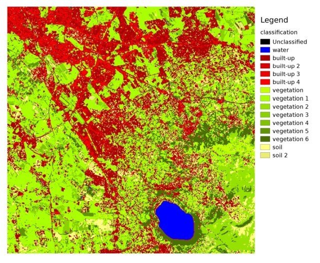
3.2.7. Resultado da Classificação ¶

O resultado do processo de classificação é um raster ( veja um exemplo de classificação Landsat na Figura v:guilabel:classificação Landsat), onde os valores de pixel correspondem a classes IDs e cada cor representa uma classe de cobertura da terra.

v:guilabel:classificação Landsat

Dados disponibilizados pelo Serviço Geológico dos EUA

Uma certa quantidade de erros podem ocorrer na classificação da cobertura da terra (i.e. pixels atribuídos a uma classe de cobertura errada), devido à similaridade espectral das classes, ou definição errada de classe durante a coleta de ROI.

3.2.8. Avaliação da Acurácia ¶

Após o processo de classificação, é útil avaliar a acurácia da classificação de cobertura da terra, buscando identificar e medir os erros do mapa. Normalmente , a avaliação da acurácia é realizada com o cálculo de uma matriz de erro, que é uma tabela que compara as informações do mapa com dados de referência (i.e. dados verdadeiros em nível de solo) para um número de áreas amostrais (Congalton e Green, 2009).

A tabela seguinte é um esquema de matriz de erro, onde k é o número de classes identificadas na classificação de cobertura da terra, e n é o número total de unidades de amostras coletadas. Os itens na diagonal maior (aii) representam o número de amostras corretamente identificadas, enquanto os outros itens são erros de classificação.

Scheme of Error Matrix

	Amostra de referência 1	Amostra de referência 2	…	Amostra de referência k	Total
Classe 1	\(a_{11}\)	\(a_{12}\)	…	\(a_{1k}\)	\(a_{1+}\)
Classe 2	\(a_{21}\)	\(a_{22}\)	…	\(a_{2k}\)	\(a_{2+}\)
…	…	…	…	…	…
Classe k	\(a_{k1}\)	\(a_{k2}\)	…	\(a_{kk}\)	\(a_{k+}\)
Total	\(a_{+1}\)	\(a_{+2}\)	…	\(a_{+k}\)	\(n\)

Portanto, é possível calcular a acurácia como um todo através da razão entre o número de amostras que são classificadas corretamente (a soma da diagonal maior), e o número total de unidades de amostra N (Congalton e Green, 2009).

Para mais informações, a documentação a seguir está disponível gratuitamente: Manual do Usuário de Dados Científicos Landsat 7, Notas de Sensoriamento Remoto , ou Wikipédia.

3.3. Image conversion to reflectance ¶

This chapter provides information about the conversion to reflectance implemented in SCP.

3.3.1. Radiance at the Sensor’s Aperture ¶

Radiance is the “flux of energy (primarily irradiant or incident energy) per solid angle leaving a unit surface area in a given direction”, “Radiance is what is measured at the sensor and is somewhat dependent on reflectance” (NASA, 2011, p. 47).

Images such as Landsat or Sentinel-2 are composed of several bands and a metadata file which contains information required for the conversion to reflectance.

Landsat images are provided in radiance, scaled prior to output. for Landsat images Spectral Radiance at the sensor’s aperture (\(L_{\lambda}\), measured in [watts/(meter squared * ster * \(\mu m\))]) is given by (https://landsat.usgs.gov/Landsat8_Using_Product.php):

\[L_{\lambda} = M_{L} * Q_{cal} + A_{L}\]

onde:

\(M_{L}\) = Band-specific multiplicative rescaling factor from Landsat metadata (RADIANCE_MULT_BAND_x, where x is the band number)
\(A_{L}\) = Band-specific additive rescaling factor from Landsat metadata (RADIANCE_ADD_BAND_x, where x is the band number)
\(Q_{cal}\) = Quantized and calibrated standard product pixel values (DN)

Sentinel-2 images (Level-1C) are already provided in Top Of Atmosphere (TOA) Reflectance, scaled prior to output (ESA, 2015).

3.3.2. Top Of Atmosphere (TOA) Reflectance ¶

Images in radiance can be converted to Top Of Atmosphere (TOA) Reflectance (combined surface and atmospheric reflectance) in order to reduce the in between-scene variability through a normalization for solar irradiance. This TOA reflectance (\(\rho_{p}\)), which is the unitless ratio of reflected versus total power energy (NASA, 2011), is calculated by:

\[\rho_{p} = (\pi * L_{\lambda} * d^{2} )/ (ESUN_{\lambda} * cos\theta_{s})\]

onde:

\(L_{\lambda}\) = Spectral radiance at the sensor’s aperture (at-satellite radiance)
\(d\) = Earth-Sun distance in astronomical units (provided with Landsat 8 metadata file, and an excel file is available from http://landsathandbook.gsfc.nasa.gov/excel_docs/d.xls)
\(ESUN_{\lambda}\) = Mean solar exo-atmospheric irradiances
\(\theta_{s}\) = Solar zenith angle in degrees, which is equal to \(\theta_{s}\) = 90° - \(\theta_{e}\) where \(\theta_{e}\) is the Sun elevation

It is worth pointing out that Landsat 8 images are provided with band-specific rescaling factors that allow for the direct conversion from DN to TOA reflectance.

Sentinel-2 images are already provided in scaled TOA reflectance, which can be converted to TOA reflectance with a simple calculation using the Quantification Value provided in the metadata (see https://sentinel.esa.int/documents/247904/349490/S2_MSI_Product_Specification.pdf).

3.3.3. Surface Reflectance ¶

The effects of the atmosphere (i.e. a disturbance on the reflectance that varies with the wavelength) should be considered in order to measure the reflectance at the ground.

As described by Moran et al. (1992), the land surface reflectance (\(\rho\)) is:

\[\rho = [\pi * (L_{\lambda} - L_{p}) * d^{2}]/ [T_{v} * ( (ESUN_{\lambda} * cos\theta_{s} * T_{z} ) + E_{down} )]\]

onde:

\(L_{p}\) is the path radiance
\(T_{v}\) is the atmospheric transmittance in the viewing direction
\(T_{z}\) is the atmospheric transmittance in the illumination direction
\(E_{down}\) is the downwelling diffuse irradiance

Therefore, we need several atmospheric measurements in order to calculate \(\rho\) (physically-based corrections). Alternatively, it is possible to use image-based techniques for the calculation of these parameters, without in-situ measurements during image acquisition. It is worth mentioning that Landsat Surface Reflectance High Level Data Products for Landsat 8 are available (for more information read http://landsat.usgs.gov/CDR_LSR.php).

3.3.4. DOS1 Correction ¶

The Dark Object Subtraction (DOS) is a family of image-based atmospheric corrections. Chavez (1996) explains that “the basic assumption is that within the image some pixels are in complete shadow and their radiances received at the satellite are due to atmospheric scattering (path radiance). This assumption is combined with the fact that very few targets on the Earth’s surface are absolute black, so an assumed one-percent minimum reflectance is better than zero percent”. It is worth pointing out that the accuracy of image-based techniques is generally lower than physically-based corrections, but they are very useful when no atmospheric measurements are available as they can improve the estimation of land surface reflectance. The path radiance is given by (Sobrino, et al., 2004):

\[L_{p} = L_{min} - L_{DO1\%}\]

onde:

\(L_{min}\) = “radiance that corresponds to a digital count value for which the sum of all the pixels with digital counts lower or equal to this value is equal to the 0.01% of all the pixels from the image considered” (Sobrino, et al., 2004, p. 437), therefore the radiance obtained with that digital count value (\(DN_{min}\))
\(L_{DO1\%}\) = radiance of Dark Object, assumed to have a reflectance value of 0.01

In particular for Landsat images:

\[L_{min} = M_{L} * DN_{min} + A_{L}\]

Sentinel-2 images are converted to radiance prior to DOS1 calculation.

The radiance of Dark Object is given by (Sobrino, et al., 2004):

\[L_{DO1\%} = 0.01 * [(ESUN_{\lambda} * cos\theta_{s} * T_{z} ) + E_{down}] * T_{v} / (\pi * d^{2})\]

Therefore the path radiance is:

\[L_{p} = M_{L} * DN_{min} + A_{L} - 0.01* [(ESUN_{\lambda} * cos\theta_{s} * T_{z} ) + E_{down}] * T_{v} / (\pi * d^{2})\]

There are several DOS techniques (e.g. DOS1, DOS2, DOS3, DOS4), based on different assumption about \(T_{v}\), \(T_{z}\) , and \(E_{down}\) . The simplest technique is the DOS1, where the following assumptions are made (Moran et al., 1992):

\(T_{v}\) = 1
\(T_{z}\) = 1
\(E_{down}\) = 0

Therefore the path radiance is:

\[L_{p} = M_{L} * DN_{min} + A_{L} - 0.01 * ESUN_{\lambda} * cos\theta_{s} / (\pi * d^{2})\]

E o resultado da reflectância da superfície da terra é dado por:

\[\rho = [\pi * (L_{\lambda} - L_{p}) * d^{2}]/ (ESUN_{\lambda} * cos\theta_{s})\]

ESUN [W /(m2 * \(\mu m\))] valores para sensores Landsat são fornecidos na tabela a seguir.

ESUN values for Landsat bands

Banda	Landsat 1 MSS*	Landsat 2 MSS*	Landsat 3 MSS*	Landsat 4 TM*	Landsat 5 TM*	Landsat 7 ETM+**
1				1983	1983	1970
2				1795	1796	1842
3				1539	1536	1547
4	1823	1829	1839	1028	1031	1044
5	1559	1539	1555	219.8	220	225.7
6	1276	1268	1291
7	880.1	886.6	887.9	83.49	83.44	82.06
8						1369

* from Chander, Markham, & Helder (2009)

** from http://landsathandbook.gsfc.nasa.gov/data_prod/prog_sect11_3.html

For Landsat 8, \(ESUN\) can be calculated as (from http://grass.osgeo.org/grass65/manuals/i.landsat.toar.html):

\[ESUN = (\pi * d^{2}) * RADIANCE\_MAXIMUM / REFLECTANCE\_MAXIMUM\]

onde RADIANCE_MAXIMUM e REFLECTANCE_MAXIMUM são fornecidos pelos metadados da imagem.

ESUN [W /(m2 * \(\mu m\))] values for Sentinel-2 sensor (provided in image metadata) are illustrated in the following table.

ESUN values for Sentinel-2 bands

Banda	Sentinel-2
1	1913.57
2	1941.63
3	1822.61
4	1512.79
5	1425.56
6	1288.32
7	1163.19
8	1036.39
8A	955.19
9	813.04
10	367.15
11	245.59
12	85.25

ESUN [W /(m2 * \(\mu m\))] values for ASTER sensor are illustrated in the following table (from Finn, et al., 2012).

ESUN values for ASTER bands

Banda	ASTER
1	1848
2	1549
3	1114
4	225.4
5	86.63
6	81.85
7	74.85
8	66.49
9	59.85

An example of comparison of to TOA reflectance, DOS1 corrected reflectance and the Landsat Surface Reflectance High Level Data Products (ground truth) is provided in Figure Spectral signatures of a built-up pixel.

Spectral signatures of a built-up pixel

Comparison of TOA reflectance, DOS1 corrected reflectance and Landsat Surface Reflectance High Level Data Products

3.4. Conversion to Temperature ¶

This chapter provides the basic information about the conversion to At-Satellite Brightness Temperature implemented in SCP and the estimation of Land Surface Temperature.

3.4.1. Conversion to At-Satellite Brightness Temperature ¶

For thermal bands, the conversion of DN to At-Satellite Brightness Temperature is given by (from https://landsat.usgs.gov/Landsat8_Using_Product.php):

\[T_{B} = K_{2} / ln[(K_{1} / L_{\lambda}) + 1]\]

onde:

\(K_{1}\) = constante de conversão termal da banda específica (em watts/metro quadrado * ster * \(\mu m\))
\(K_{2}\) = constante de conversão termal da banda específica (em kelvin)

and \(L_{\lambda}\) is the Spectral Radiance at the sensor’s aperture, measured in watts/(meter squared * ster * \(\mu m\)).

The \(K_{1}\) and \(K_{2}\) constants for Landsat sensors are provided in the following table.

Thermal Conversion Constants for Landsat

Constante	Landsat 4*	Landsat 5*	Landsat 7**
\(K_{1}\)	671.62	607.76	666.09
\(K_{2}\)	1284.30	1260.56	1282.71

* de Chander & Markham (2003)

** da NASA (2011)

For Landsat 8, the \(K_{1}\) and \(K_{2}\) values are provided in the image metadata file.

\(K_{1}\) and \(K_{2}\) are calculated as (Jimenez-Munoz & Sobrino, 2010):

\[K_{1} = c_{1} / \lambda^{5}\]

\[K_{2} = c_{2} / \lambda\]

where (Mohr, Newell, & Taylor, 2015):

\(c_{1}\) = first radiation constant = \(1.191 * 10^{-16} W m^{2} sr^{-1}\)
\(c_{2}\) = second radiation constant = \(1.4388 * 10^{-2} m K\)

Therefore, for ASTER bands \(K_{1}\) and \(K_{2}\) are provided in the following table.

Thermal Conversion Constants for ASTER

Constante	Band 10	Band 11	Band 12	Band 13	Band 14
\(K_{1}\)	\(3.024 * 10^{3}\)	\(2.460 * 10^{3}\)	\(1.909 * 10^{3}\)	\(8.900 * 10^{2}\)	\(6.464 * 10^{2}\)
\(K_{2}\)	\(1.733 * 10^{3}\)	\(1.663 * 10^{3}\)	\(1.581 * 10^{3}\)	\(1.357 * 10^{3}\)	\(1.273 * 10^{3}\)

3.4.2. Estimation of Land Surface Temperature ¶

Several studies have described the estimation of Land Surface Temperature. Land Surface Temperature can be calculated from At-Satellite Brightness Temperature \(T_{B}\) as (Weng, et al. 2004):

\[T = T_{B} / [ 1 + (\lambda * T_{B} / c_{2}) * ln(e) ]\]

onde:

\(\lambda\) = wavelength of emitted radiance
\(c_{2} = h * c / s = 1.4388 * 10^{-2}\) m K
\(h\) = Planck’s constant = \(6.626 * 10^{-34}\) J s
\(s\) = Boltzmann constant = \(1.38 * 10^{-23}\) J/K
\(c\) = velocity of light = \(2.998 * 10^{8}\) m/s

The values of \(\lambda\) for the thermal bands of Landsat and ASTER satellites can be calculated from the tables in Satélite Landsat and ASTER Satellite.

Several studies used NDVI for the estimation of land surface emissivity (Sobrino, et al., 2004); other studies used a land cover classification for the definition of the land surface emissivity of each class (Weng, et al. 2004). For instance, the emissivity (\(e\)) values of various land cover types are provided in the following table (from Mallick, et al. 2012).

Emissivity values

Land surface	Emissivity e
Solo	0.928
Gramado	0.982
Asphalt	0.942
Concrete	0.937

3.5. References ¶

Chander, G. & Markham, B. 2003. Revised Landsat-5 TM radiometric calibration procedures and postcalibration dynamic ranges Geoscience and Remote Sensing, IEEE Transactions on, 41, 2674 - 2677
Chavez, P. S. 1996. Image-Based Atmospheric Corrections - Revisited and Improved Photogrammetric Engineering and Remote Sensing, [Falls Church, Va.] American Society of Photogrammetry, 62, 1025-1036
Congalton, R. and Green, K., 2009. Assessing the Accuracy of Remotely Sensed Data: Principles and Practices. Boca Raton, FL: CRC Press
Didan, K.; Barreto Munoz, A.; Solano, R. & Huete, A. 2015. MODIS Vegetation Index User’s Guide. Collection 6, NASA
ESA. Manual do Usuário Sentinel-2. 2015. Disponível em: https://sentinel.esa.int/documents/247904/685211/Sentinel-2_User_Handbook.
Finn, M.P., Reed, M.D, and Yamamoto, K.H. 2012. A Straight Forward Guide for Processing Radiance and Reflectance for EO-1 ALI, Landsat 5 TM, Landsat 7 ETM+, and ASTER. Unpublished Report from USGS/Center of Excellence for Geospatial Information Science, 8 p, http://cegis.usgs.gov/soil_moisture/pdf/A%20Straight%20Forward%20guide%20for%20Processing%20Radiance%20and%20Reflectance_V_24Jul12.pdf
Fisher, P. F. and Unwin, D. J., eds. 2005. Representing GIS. Chichester, England: John Wiley & Sons
JARS. Notas de Sensoriamento Remoto. Associação Japonesa de Sensoriamento Remoto. 1993. Disponível em: http://www.jars1974.net/pdf/rsnote_e.html
Jimenez-Munoz, J. C. & Sobrino, J. A. 2010. A Single-Channel Algorithm for Land-Surface Temperature Retrieval From ASTER Data IEEE Geoscience and Remote Sensing Letters, 7, 176-179
Johnson, B. A., Tateishi, R. and Hoan, N. T. Imagem de Satélite Pansharpening Usando uma Abordagem Híbrida Baseada em Objeto para Análise de Imagem ISPRS. International Journal of Geo-Information, 1, 228. 2012. Disponível em: http://www.mdpi.com/2220-9964/1/3/228)
Kruse, F. A., et al., 1993. The Spectral Image Processing System (SIPS) - Interactive Visualization and Analysis of Imaging spectrometer. Data Remote Sensing of Environment
Mallick, J.; Singh, C. K.; Shashtri, S.; Rahman, A. & Mukherjee, S. 2012. Land surface emissivity retrieval based on moisture index from LANDSAT TM satellite data over heterogeneous surfaces of Delhi city International Journal of Applied Earth Observation and Geoinformation, 19, 348 - 358
Mohr, P. J.; Newell, D. B. & Taylor, B. N. 2015. CODATA Recommended Values of the Fundamental Physical Constants: 2014 National Institute of Standards and Technology, Committee on Data for Science and Technology
Moran, M.; Jackson, R.; Slater, P. & Teillet, P. 1992. Evaluation of simplified procedures for retrieval of land surface reflectance factors from satellite sensor output Remote Sensing of Environment, 41, 169-184
NASA (Ed.) 2011. Landsat 7 Science Data Users Handbook Landsat Project Science Office at NASA’s Goddard Space Flight Center in Greenbelt, 186 http://landsathandbook.gsfc.nasa.gov/pdfs/Landsat7_Handbook.pdf
NASA. Manual do Usuário de Dados Científicos Landsat 7. 2013. Disponível em: http://landsathandbook.gsfc.nasa.gov
Ready, P. and Wintz, P., 1973. Information Extraction, SNR Improvement, and Data Compression in Multispectral Imagery. IEEE Transactions on Communications, 21, 1123-1131
Richards, J. A. and Jia, X. Análise de Imagem Digital de Sensoriamento Remoto: Uma Introdução. Berlim, Alemanha: Springer, 2006.
Sobrino, J.; Jiménez-Muñoz, J. C. & Paolini, L. A reobtenção da temperatura da superfície da terra de uma Landsat TM 5 Sensoriamento Remoto do Ambiente, Elsevier, 90, 434-440. 2004
USGS, 2015. Advanced Spaceborne Thermal Emission and Reflection Radiometer (ASTER) Level 1 Precision Terrain Corrected Registered At-Sensor Radiance Product (AST_L1T). AST_L1T Product User’s Guide. USGS EROS Data Center.
Vermote, E. F.; Roger, J. C. & Ray, J. P. 2015. MODIS Surface Reflectance User’s Guide. Collection 6, NASA
Weng, Q.; Lu, D. & Schubring, J. 2004. Estimation of land surface temperature–vegetation abundance relationship for urban heat island studies. Remote Sensing of Environment, Elsevier Science Inc., Box 882 New York NY 10159 USA, 89, 467-483