5.2. Tutorial: Estimation of Land Surface Temperature with Landsat and ASTER

This tutorial is about the estimation land surface temperature using Satélite Landsat and Satélite ASTER images. In this tutorial we are going to use a land cover classification for the definition of surface emissivity, which is required for the calculation of the land surface temperature. It is assumed that one has the basic knowledge of SCP and Tutoriales Básicos.

Our study area will be Paris (France), an area covered by urban surfaces, vegetation and agricultural fields.

Before downloading data, please watch the following video that illustrates the study area and provides very useful information about thermal infrared images, and their application (footage courtesy of European Space Agency/ESA). Also, a brief description of the area that we are going to classify is available here .

http://www.youtube.com/watch?v=Vjg5REQb-Bc

The thermal infrared band is particularly useful for assessing the temperature difference between the city and the surrounding rural areas, and studying the urban heat island phenomenon. We are going to use Landsat and ASTER images for the estimation of land surface temperature. For more information about the conversion of raster bands please read Conversión a Temperatura de Brillo en el Satélite. Following the video of this tutorial.

http://www.youtube.com/watch?v=7W4IwlvPLbQ

5.2.1. Data Download and Conversion

We are going to download the Landsat 8 image acquired in 2015 (image ID = LC81990262015270LGN00, data available from the U.S. Geological Survey).

Start a new QGIS project. Open the tab Descarga de Imágenes clicking the button in the SCP menú, or the SCP Herramientas, or the SCP panel. Select the tab Descargar Landsat.

In Acceso https://ers.cr.usgs.gov/ you should enter the user name and password for accessing data (free registration at USGS EROS is required) in User and Password. However, in this case login should not be required because this Landsat 8 image is available directly from the Amazon Web Services (AWS) .

In Area de búsqueda enter:

• UL X (Lon): 2

• UL Y (Lat): 49

• LR X (Lon): 2.5

• LR Y (Lat): 48.8

  Consejo : En general es posible definir las coordenadas del area pulsando sobre el boton y dibujando un rectangulo en el mapa.

In Buscar select L8 OLI/TIRS from the list Satellites and set the acquisition date:

• Date from: 2015-09-27
• to: 2015-09-27

Ahora pulsa el botón Buscar y luego de unos segundos la imagen se mostrará en la lista de imágenes.

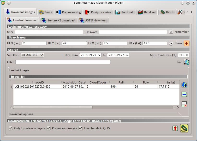
Landsat search result

In the result table, click the item LC81990262015270LGN00 in the field ImageID, and click the button . A preview will be downloaded and displayed in the map, which is useful for assessing the quality of the image and the cloud cover.

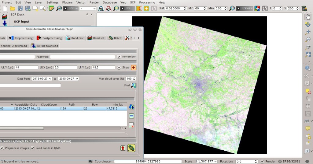
Vista previa de la imagen

Click the tab Opciones de Descarga and leave checked only the following bands:

• 2 = Blue
• 3 = Green
• 4 = Red
• 5 = Near-Infrared
• 6 = Short Wavelength Infrared 1
• 7 = Short Wavelength Infrared 2
• 10 = Thermal Infrared (TIRS) 1

Bands from 2 to 7 will be used for the land cover classification, and band 10 for the estimation of land surface temperature (see ¿Por qué solo usar la banda 10 del Landsat 8 en la estimación de la temperatura de la superficie?).

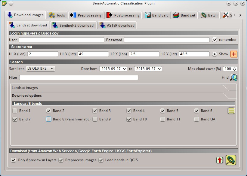
Selección de bandas a descargar

The checkbox Preprocess images allows for the automatic conversion of bands after the download, according to the settings defined in Landsat; we are going to apply the Corrección DOS1. Bands from 2 to 7 will be converted to reflectance and band 10 will be converted to At-Satellite Brightness Temperature. Open the tab Landsat, check Apply DOS1 atmospheric correction and uncheck Create Band set and use Band set tools (we are going to create the Band set after the clip of the image to study area).

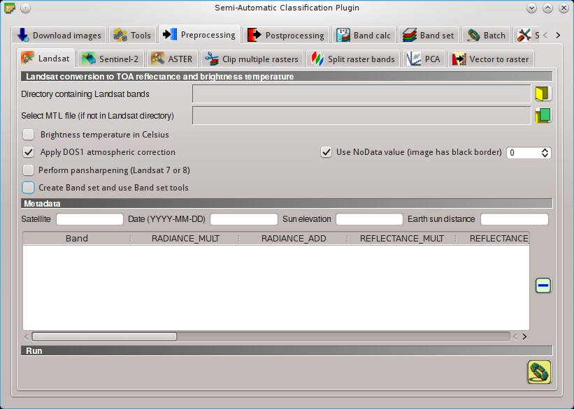
Conversion settings

In order to start the download and conversion process, open the tab Descargar Landsat, click the button and select the directory where converted bands are saved (e.g. Desktop). After a few minutes, converted bands are loaded and displayed (file name starts with RT_).

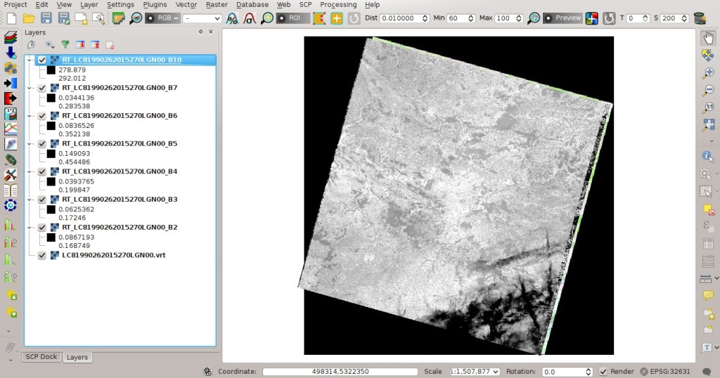
Converted Landsat bands

5.2.2. Clip to Study Area

We are going to clip the Landsat images to our study area.

Open the tab Preprocesamiento clicking the button in the SCP menú, or the SCP Herramientas, or the SCP panel. Select the tab Recortar múltiples rásters and click the button to refresh the layer list and show the loaded rasters. Click the button to select all the rasters to be clipped, and in Coordenadas de corte type the following values:

• UL X: 402705
• UL Y: 5461065
• LR X: 480824
• LR Y: 5381535

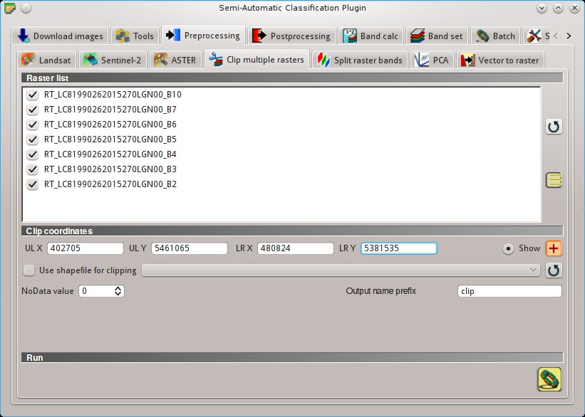
Recortar área

Now click the button and select the directory where clipped bands are saved (e.g. Desktop). Clipped bands have the prefix clip_ and will be automatically loaded and displayed. We can remove the bands whose names start with RT_ from QGIS layers.

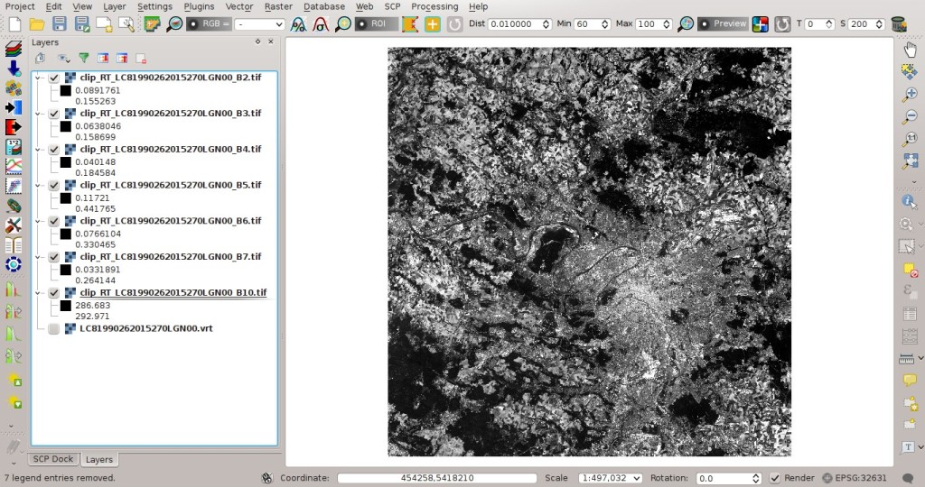
Bandas recortadas

5.2.3. Land Cover Classification

Now we need to classify land cover, which will be used later for the creation of the emissivity raster. For detailed instructions about the classification process please see Tutorial 2: Clasificación de la Cobertura del Suelo con Imágenes de Sentinel-2.

We are going to use the following Macroclass IDs (see Clases y Macroclases).

Macroclases

Nombre de la Macroclase	Macroclase ID
Agua	1
Construcciones	2
Vegetación	3
Suelo	4

Open the tab Conjunto de bandas clicking the button and define the Landsat 8 Band set using clipped bands from 2 to 7 (excluding band 10).

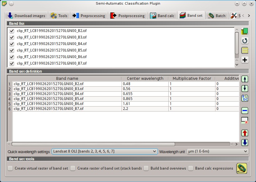
Conjunto de bandas

In the SCP panel click the button , define a file name for the Training input. In the list RGB= of Barra de Trabajo select 4-3-2 to display a false color composite corresponding to the bands: Near-Infrared, Red, and Green (see Composición de Color).

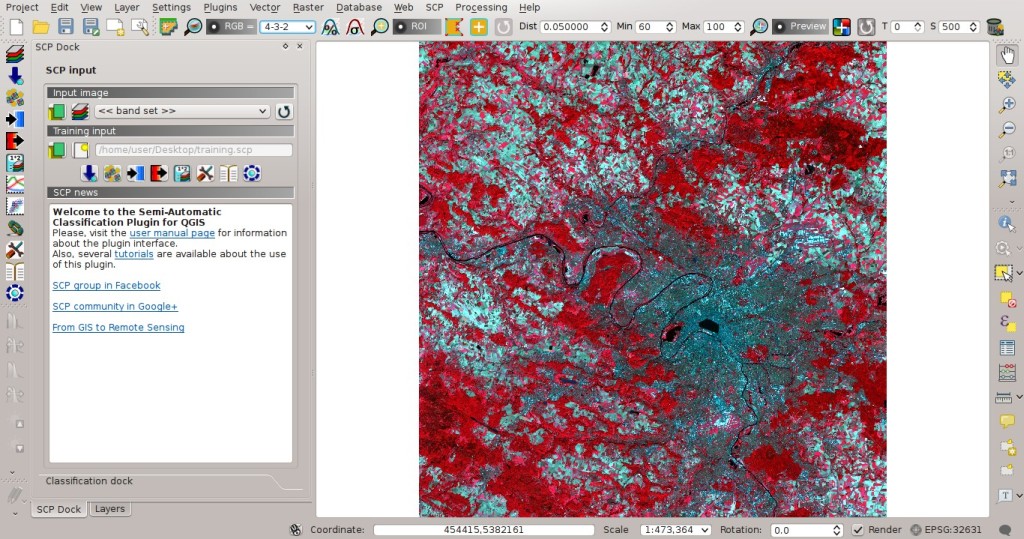
Color composite

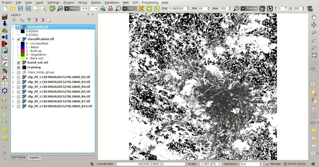
After the creation of several ROIs for each land cover class, we can perform the classification of the whole image (see Tutorial 2: Clasificación de la Cobertura del Suelo con Imágenes de Sentinel-2). After setting the colors of MC ID (in the tab Macroclasses of the SCP panel), in the tab Classification algorithm check the option MC ID to use Macroclass IDs and select the classification algorithm Máxima Probabilidad.

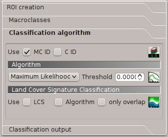
Classification algorithm

Then, open the tab Classification output, click the button and define the name of the classification output.

Land cover classification

5.2.4. Reclassification of Land Cover Classification to Emissivity Values

Now we are going to reclassify the classification raster using the land surface emissivity values. The emissivity (e) values for the land cover classes are provided in the following table (values used in this tutorial are only indicative, because emissivity of every material should be obtained from field survey):

Valores de emisividad

Superficie de la tierra	Emisividad e
Agua	0.98
Construcciones	0.94
Vegetación	0.98
Suelo	0.93

Open the tab Postprocesamiento clicking the button in the SCP menú, or the SCP Herramientas, or the SCP panel. Select the tab Reclasificación and click the button to refresh the layer list and show the loaded rasters. Select the classification raster from the list.

Click the button to add 4 rows to the table Values. In this table, set the old value (the Macroclass ID of the classification) and the new value (the corresponding emissivity e ) for every land cover class. Uncheck the checkbox Use code from Signature list, click the button and define the name of the output raster (e.g. emissivity.tif).

Reclassification

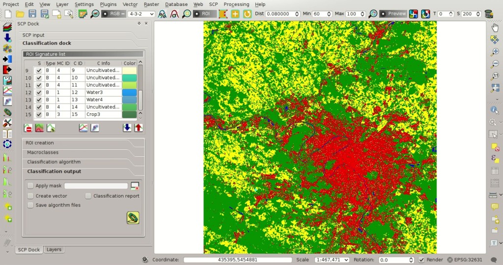
This is the emissivity raster, where each pixel has the emissivity value that we have defined for the respective land cover class.

Emissivity raster

5.2.5. Conversion from At-Satellite Temperature to Land Surface Temperature

Now we are ready to convert the At-Satellite Brightness Temperature to Land Surface Temperature, using the following equation (see Estimación de la Temperatura de Superficie del Suelo):

\[T = T_{B} / [ 1 + (\lambda * T_{B} / c_{2}) * ln(e) ]\]

donde:

• \(\lambda\) = longitud de onda de la radiancia emitida

• \(c_{2} = h * c / s = 1.4388 * 10^{-2}\) m K = 14388 µm K

• \(h\) = Constante de Planck’s = \(6.626 * 10^{-34}\) J s

• \(s\) = constante de Boltzmann = \(1.38 * 10^{-23}\) J/K

• \(c\) = velocidad de la luz \(2.998 * 10^{8}\) m/s

The values of \(\lambda\) for Landsat bands are listed in the following table.

Center wavelength of Landsat bands

Satélite	Banda	\(\lambda (µm)\)
Landsat 4, 5, and 7	6	11.45
Landsat 8	10	10.8
Landsat 8	11	12

Open the tab Calculadora de Bandas clicking the button in the SCP menú, or the SCP Herramientas, or the SCP panel. Click the button to refresh the layer list and show the loaded rasters. We have used band 10 of Landsat 8, therefore in the Expresión type the equation for conversion adapted to our rasters:

"clip_RT_LC81990262015270LGN00_B10.tif" / ( 1 + ( 10.8 * "clip_RT_LC81990262015270LGN00_B10.tif" / 14388 ) * ln("emissivity.tif") )

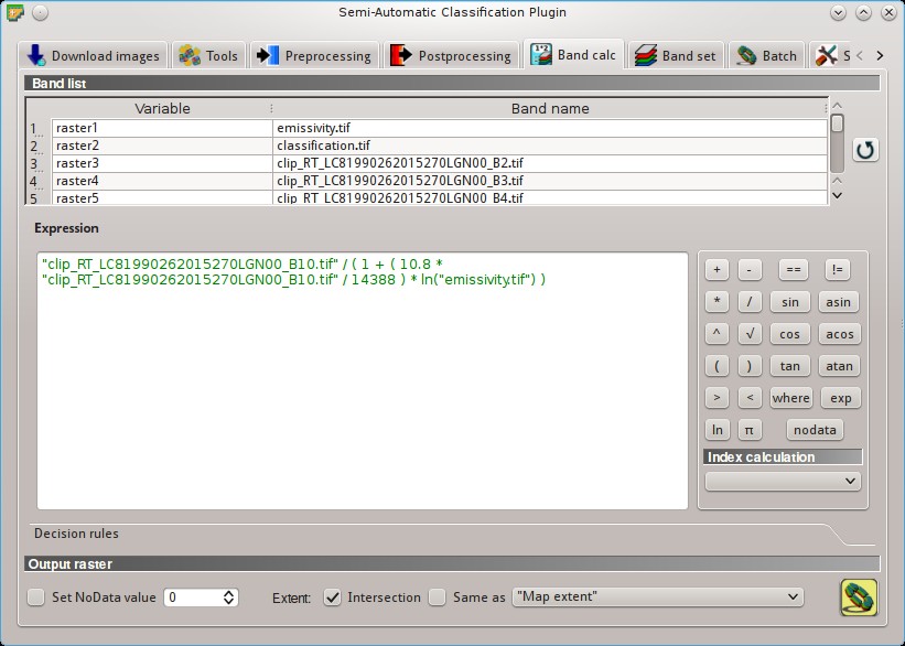
Calculation of surface temperature

Click the button and define the name of the output raster (e.g. surface_temperature.tif). After the calculation, the Land Surface Temperature (in kelvin) will be loaded, and we can change the layer style. In addition, in the tab Calculadora de Bandas we can calculate the temperature in Celsius with the expression:

"surface_temperature.tif" - 273.15

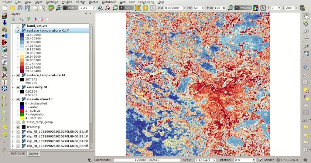
Land Surface Temperature of the Landsat Image

We can notice that the urban area and uncultivated land have the highest temperatures, while vegetation has the lowest temperature. The aim of this tutorial is to describe a methodology for the estimation of surface temperature using open source programs and free images. It is worth highlighting that in order to achieve more accurate results, one should perform field survey for improving the land cover classification and the estimation of surface emissivities.

In addition to Landsat, we are going to use an ASTER image and use the same methodology for the estimation of Land Surface Temperature.

5.2.6. Data Download and Conversion of ASTER Image

Open the tab Descarga de Imágenes and select the tab Descargar ASTER.

In Acceso https://urs.earthdata.nasa.gov enter the user name and password required for accessing data (free registration at EOSDIS Earthdata is required) in User and Password. The ASTER L1T data products are retrieved from the online Data Pool, courtesy of the NASA Land Processes Distributed Active Archive Center (LP DAAC), USGS/Earth Resources Observation and Science (EROS) Center, Sioux Falls, South Dakota, https://lpdaac.usgs.gov/data_access/data_pool.

In Area de búsqueda enter:

• UL X (Lon): 2
• UL Y (Lat): 49
• LR X (Lon): 2.5
• LR Y (Lat): 48.8

In Buscar set the acquisition date:

• Date from: 2000-08-24
• to: 2000-08-24

Ahora pulsa el botón Buscar y luego de unos segundos la imagen se mostrará en la lista de imágenes.

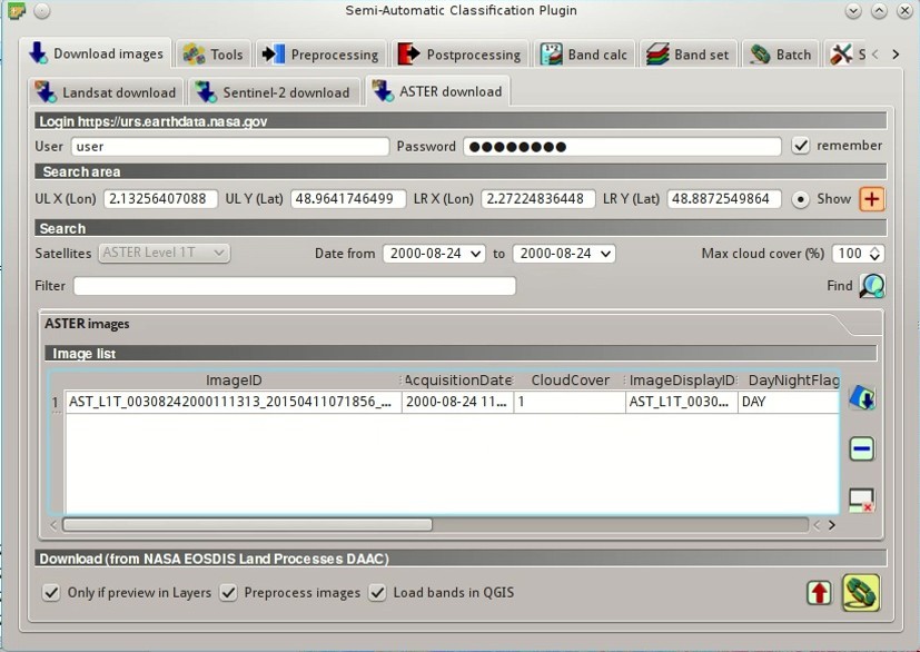
ASTER search result

In the result table, click the item AST_L1T_00308242000111313_20150411071856_3805 in the field ImageID, and click the button . A preview will be downloaded and displayed in the map, which is useful for assessing the quality of the image and the cloud cover.

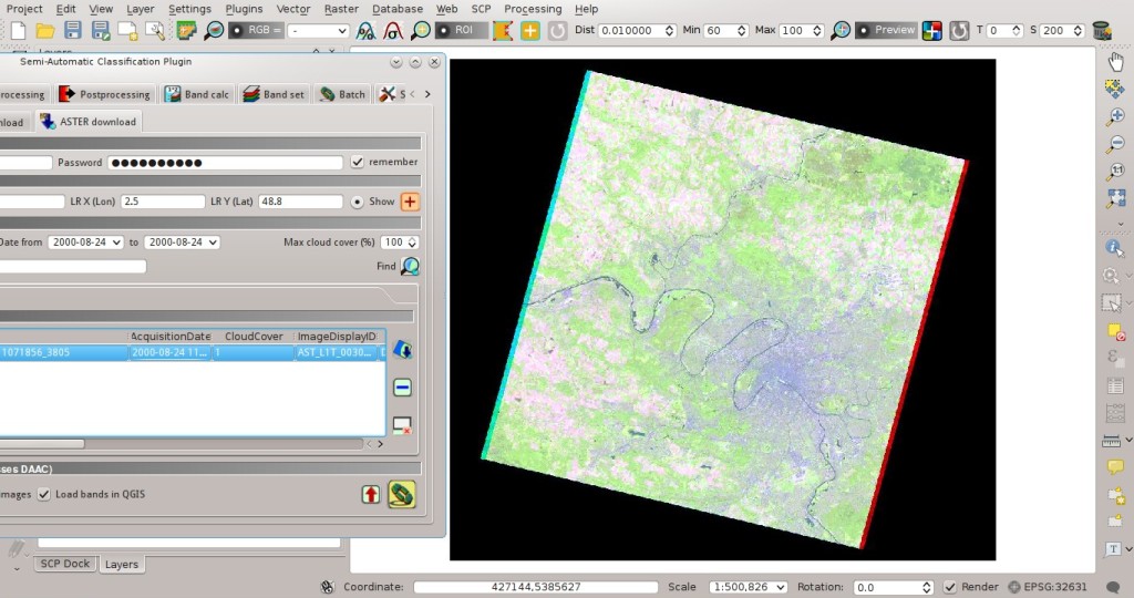
ASTER image preview

As we did for Landsat, we are going to apply the Corrección DOS1. The checkbox Preprocess images allows for the automatic conversion of bands after the download, according to the settings defined in ASTER. Bands from 1 to 9 will be converted to reflectance and bands from 10 to 14 will be converted to At-Satellite Brightness Temperature.

Open the tab ASTER, check Apply DOS1 atmospheric correction and leave checked Create Band set and use Band set tools (this is useful to automatiacally create a Band set, which is required for the next step).

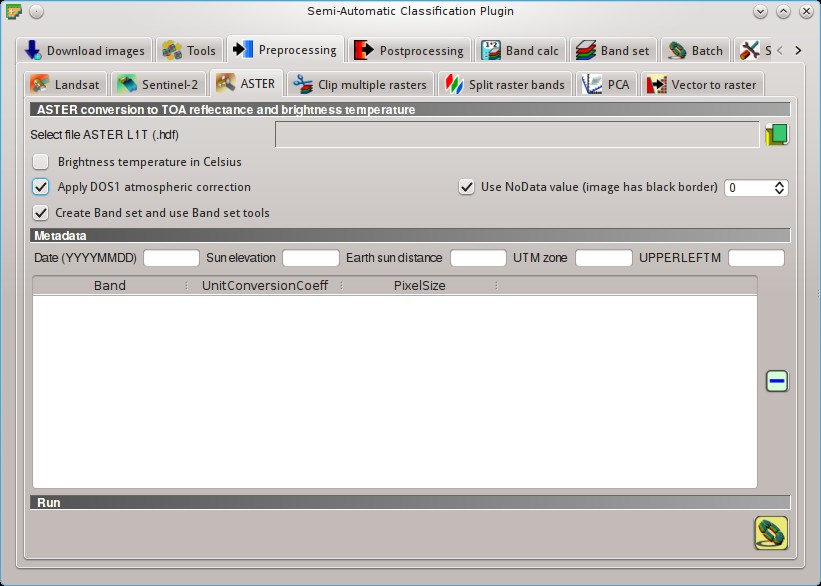
Conversion settings

In order to start the download and conversion process, open the tab Descargar ASTER, click the button and select the directory where converted bands are saved (e.g. Desktop). After a few minutes, converted bands are loaded and displayed (file name starts with RT_).

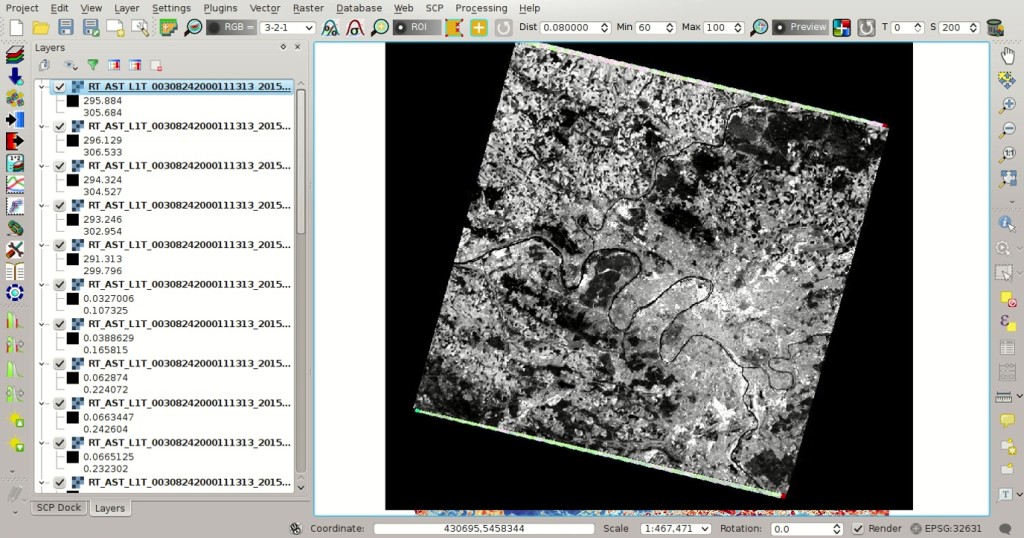
Converted ASTER bands

5.2.7. Clip to Study Area of ASTER image

We are going to clip the ASTER images to our study area, because bands are not aligned at the border.

Open the tab Preprocesamiento clicking the button . Select the tab Recortar múltiples rásters and click the button to refresh the layer list and show the loaded rasters. Band set`Click the button |select_all| to select all the rasters to be clipped, and check |checkbox| :guilabel:`Use temporary ROI for clipping. Now, we can draw a manual ROI (because a Band set is already defined, see ROI creación de) about the same shape of the ASTER image, about 20 pixels within the border thereof (in order to align the border of all the bands).

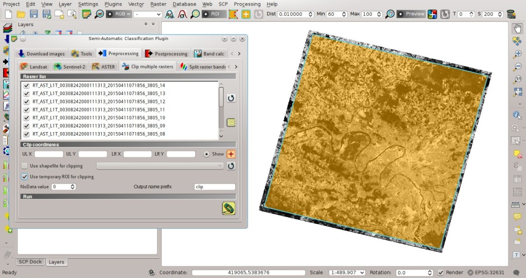
Recortar área

Now click the button and select the directory where clipped bands are saved (e.g. Desktop). Clipped bands have the prefix clip_ and will be automatically loaded and displayed. We can remove the bands whose names start with RT_ from QGIS layers.

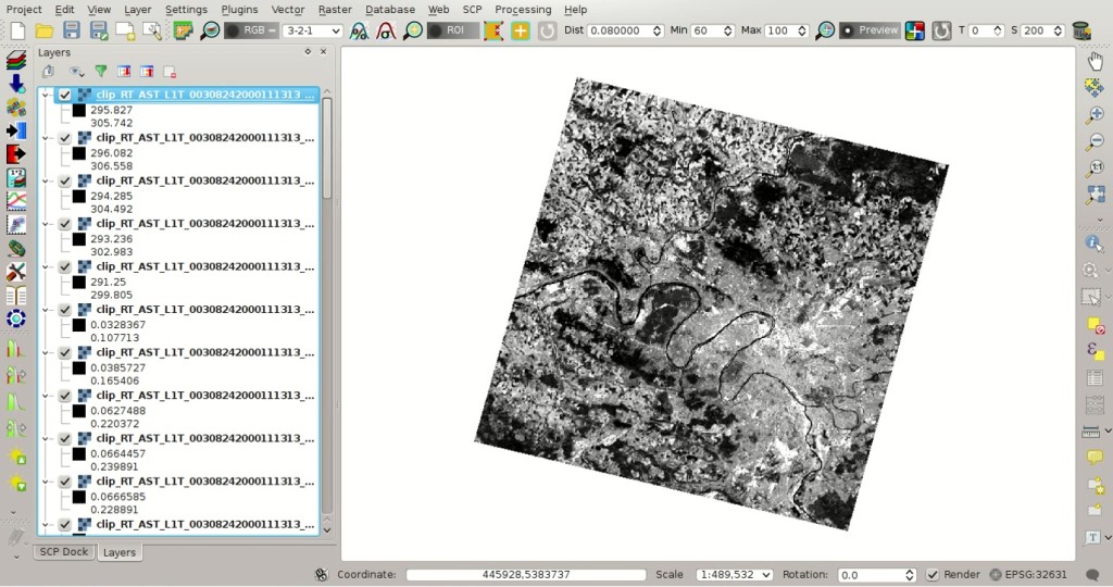
Bandas recortadas

5.2.8. Land Cover Classification of ASTER Image

Using the same Macroclass IDs used for Landsat, we are going to classify the ASTER image.

Open the tab Conjunto de bandas clicking the button . Click tha button to clear all bands from Band set and define the ASTER Band set using the clipped bands from 1 to 9.

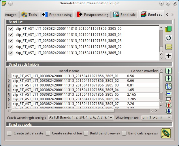
ASTER band set

In the SCP panel click the button , define a file name for the Training input (e.g. training_ASTER). Clear the table ROI Signature list highlighting all the spectral signatures created previously for Landsat and clicking the button .

In the list RGB= of Barra de Trabajo select 3-2-1 to display a false color composite corresponding to the bands: Near-Infrared, Red, and Green (see Composición de Color).

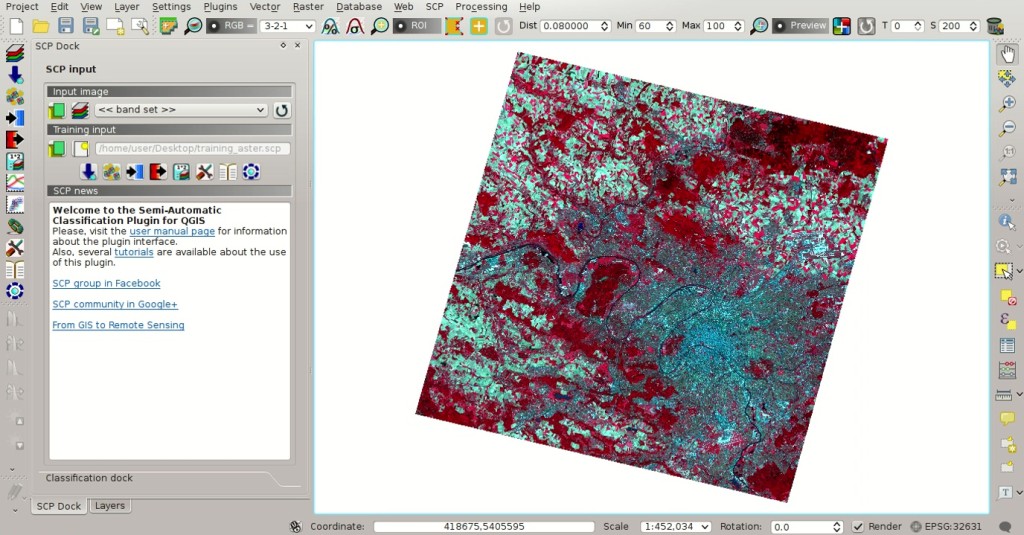
ASTER color composite

After the creation of several ROIs for each land cover class, we can perform the classification of the whole image. After setting the colors of MC ID (in the tab Macroclasses of the SCP panel), in the tab Classification algorithm check the option MC ID to use Macroclass IDs and select the classification algorithm Máxima Probabilidad. Then, open the tab Classification output, click the button and define the name of the classification output (e.g. classification_aster.tif).

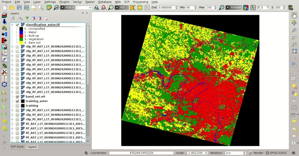
ASTER land cover classification

5.2.9. Reclassification of Land Cover Classification to Emissivity Values of ASTER Image

Now we are going to reclassify the classification raster using the same land surface emissivity values used for Landsat.

Open the tab Postprocesamiento clicking the button . Select the tab Reclasificación and click the button to refresh the layer list and show the loaded rasters. Select the classification raster from the list.

Click the button to add 4 rows to the table Values. In this table, set the old value (the Macroclass ID of the classification) and the new value (the corresponding emissivity e ) for every land cover class. Uncheck the checkbox Use code from Signature list, click the button and define the name of the output raster (e.g. emissivity_aster.tif).

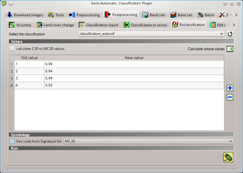
ASTER reclassification

The following figure show the emissivity raster of ASTER image.

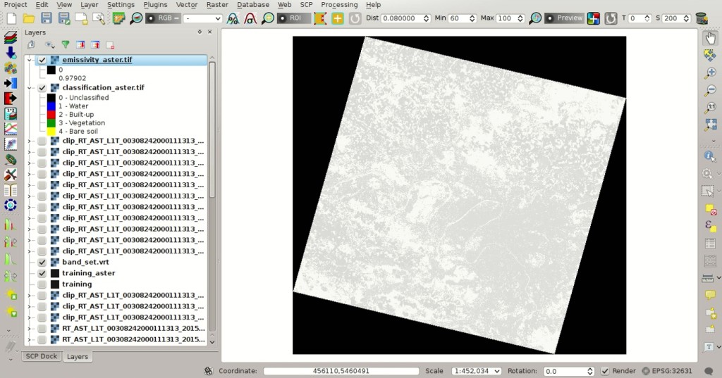
ASTER emissivity raster

5.2.10. Conversion from At Satellite Temperature to Land Surface Temperature of ASTER Image

We can convert the At-Satellite Brightness Temperature to Land Surface Temperature, using the same equation used for Landsat (see Estimación de la Temperatura de Superficie del Suelo).

The values of \(\lambda\) for ASTER bands are listed in the following table.

Center wavelength of ASTER bands

Satélite	Banda	\(\lambda (µm)\)
ASTER	10	8.3
ASTER	11	8.65
ASTER	12	9.1
ASTER	13	10.6
ASTER	14	11.3

We are going to use ASTER band 13 that has a \(\lambda\) value very similar to the Landsat band 10.

Open the tab Calculadora de Bandas clicking the button . Click the button to refresh the layer list and show the loaded rasters, and in the Expresión type equation for conversion adapted to our rasters:

"clip_RT_AST_L1T_00308242000111313_20150411071856_3805_13.tif" / ( 1 + ( 10.6 * "clip_RT_AST_L1T_00308242000111313_20150411071856_3805_13.tif" / 14388 ) * ln("emissivity_aster.tif") )

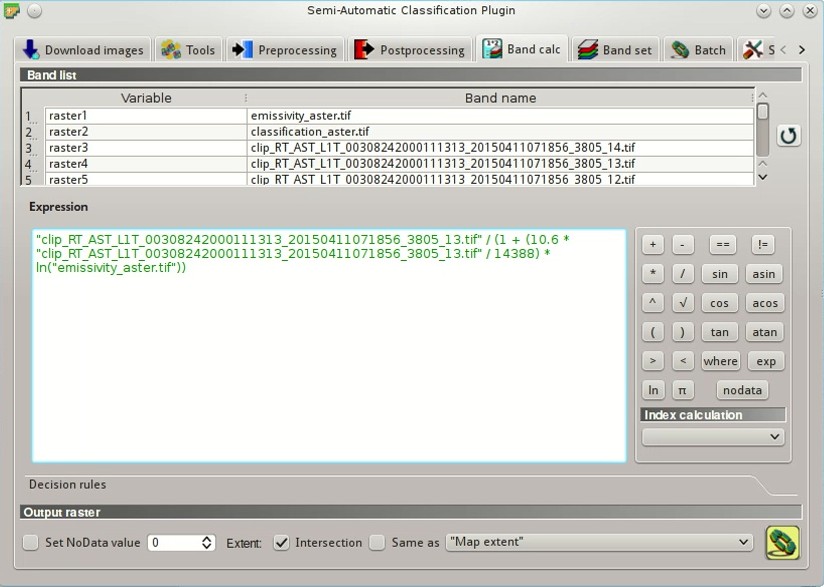
Calculation of surface temperature

Click the button and define the name of the output raster (e.g. surface_temperature_aster.tif). After the calculation, the Land Surface Temperature (in kelvin) will be loaded, and we can change the layer style. In addition, in the tab Calculadora de Bandas we can calculate the temperature in Celsius with the expression:

"surface_temperature_aster.tif" - 273.15

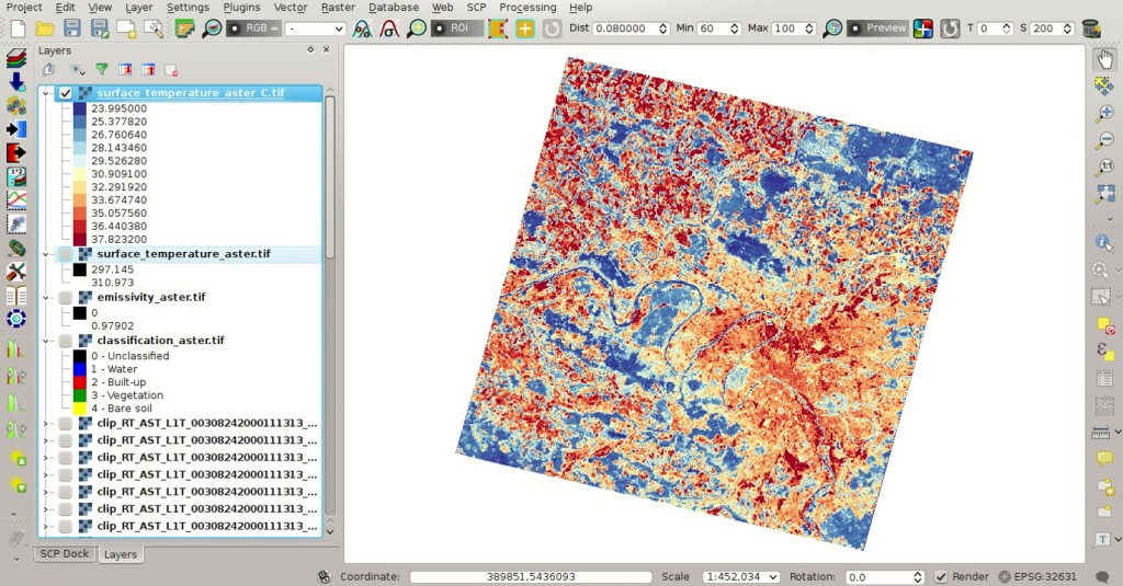
Land Surface Temperature of the ASTER Image

The ASTER image shows temperature values higher than the Landsat image. For instance, we could perform the difference between the two surface temperature rasters (Landsat and ASTER) to assess the variation of temperature. However, we should notice that the two images were acquired in different months (Landsat on 27-09-2015 and ASTER on 24-08-2000).

The large availability of Landsat and ASTER images for the past decades allows for the reliable monitoring of land cover and surface temperature. Nevertheless, cloud cover can limit the number of images that can be effectively used.

This tutorial illustrated a methodology of temperature estimation using these satellite images and open source programs. One should always consider that the estimation accuracy depends on several factors, such as the thematic and spatial accuracy of land cover classifications and the reliability of the emissivity values. Estimation errors can be of 1 K or even more. Other methods have been developed which can provide more accurate results, and the reader can continue the research.

5.2.11. Otros Tutoriales

For other tutorials visit the blog From GIS to Remote Sensing .